Managing Large-Scale Diffusion Tensor MRI Datasets: A Comprehensive Guide for Behavioral Research and Drug Development

Abstract

This article provides a comprehensive framework for handling the unique challenges posed by large Diffusion Tensor Imaging (DTI) datasets in behavioral studies and drug development research. Covering the entire data lifecycle, we explore DTI fundamentals and the specific nature of big DTI data, methodological approaches for acquisition and analysis, troubleshooting for common artifacts and performance bottlenecks, and validation strategies for multi-center studies. With a focus on practical implementation, we discuss advanced techniques including deep learning acceleration, data harmonization methods, and quality control protocols to ensure reproducible and clinically translatable results. This guide equips researchers and pharmaceutical professionals with the knowledge to optimize DTI workflows from data acquisition through analysis in large-scale studies.

Understanding DTI Fundamentals and Large-Scale Data Challenges

Core Principles & Quantitative Metrics

Frequently Asked Questions

What is the fundamental physical principle behind DTI? Diffusion Tensor Imaging (DTI) measures the Brownian motion (random thermal motion) of water molecules within biological tissues [1]. This movement is not always uniform (isotropic); in structured tissues like white matter, the parallel bundles of axons and their myelin sheaths restrict water diffusion, making it directionally dependent (anisotropic) [2] [1]. DTI quantifies this directionality and magnitude of water diffusion to infer microscopic structural details about tissue architecture.

What does the "Tensor" in DTI represent? The tensor is a 3x3 symmetric matrix that mathematically models the local diffusion properties of water in three-dimensional space within each voxel (volume element) of an image [3]. This model allows for the calculation of both the degree of anisotropy and the primary direction of diffusion, providing a more complete picture than a single scalar value [1].

How is the health of a white matter tract reflected in DTI metrics? Changes in DTI metrics are highly sensitive to microstructural alterations. For example, a decrease in Fractional Anisotropy (FA) or an increase in Mean Diffusivity (MD) often indicates axonal injury or loss of structural integrity, which can occur in conditions like traumatic brain injury [1]. Radial diffusivity is particularly associated with myelin pathology, often increasing with demyelination [1].

Quantitative DTI Metrics Table

The following table summarizes the key quantitative metrics derived from DTI, which are essential for analyzing large datasets in research.

Metric	Acronym	Description	Typical Change in Pathology
Fractional Anisotropy	FA	Quantifies the directionality of water diffusion (0=isotropic, 1=anisotropic) [1].	Decrease (e.g., axonal damage) [1].
Mean Diffusivity	MD	Represents the average rate of molecular diffusion, also known as Apparent Diffusion Coefficient (ADC) [1].	Increase (e.g., edema, necrosis) [1].
Axial Diffusivity	AD	Measures the rate of diffusion parallel to the primary axis of the axon [1].	Increase with axonal degeneration [1].
Radial Diffusivity	RD	Measures the rate of diffusion perpendicular to the primary axon direction [1].	Increase with demyelination [1].

Experimental Protocols & Data Handling

Frequently Asked Questions

What is a major data quality concern in DTI acquisition and how can it be mitigated? DTI data, often acquired using Single-shot Echo Planar Imaging (EPI), is susceptible to artifacts from eddy currents and patient motion due to its low signal-to-noise ratio (SNR) and long scan times [3]. Mitigation strategies include:

• Using parallel imaging techniques (e.g., SENSE, GRAPPA) to shorten the readout time, which reduces sensitivity to motion and geometric distortions [3].
• Increasing the number of diffusion gradient directions (e.g., 6, 9, 33, or more) to increase confidence in the accuracy of the tensor estimation, though this trades off with longer scan times [1].

Our analysis shows low anisotropy in a voxel. Does this always mean the tissue is disorganized? Not necessarily. A voxel showing low anisotropy (isotropy) may contain multiple highly anisotropic structures (e.g., crossing fibers) oriented in different directions, which cancel each other out on a macroscopic scale [1]. This is a key limitation of the standard DTI model and a primary challenge when working with complex white matter architecture in large datasets.

What are the main methods for quantitative analysis of DTI data? There are three primary methodologies, each with strengths for different research questions:

• Region of Interest (ROI): Manual or semi-automated tracing of specific brain regions for analysis. It is reliable and replicable but can be time-consuming [1].
• Whole-Brain Voxel-Based Analysis (VBA): An automated approach that performs a voxel-wise comparison across the entire brain, ideal for large-scale dataset analysis without a priori hypotheses [1].
• Tract-Based Spatial Statistics (TBSS): A "skeletonized" approach that projects all subjects' FA data onto a common white matter skeleton, reducing alignment issues and is highly popular for group studies [1].

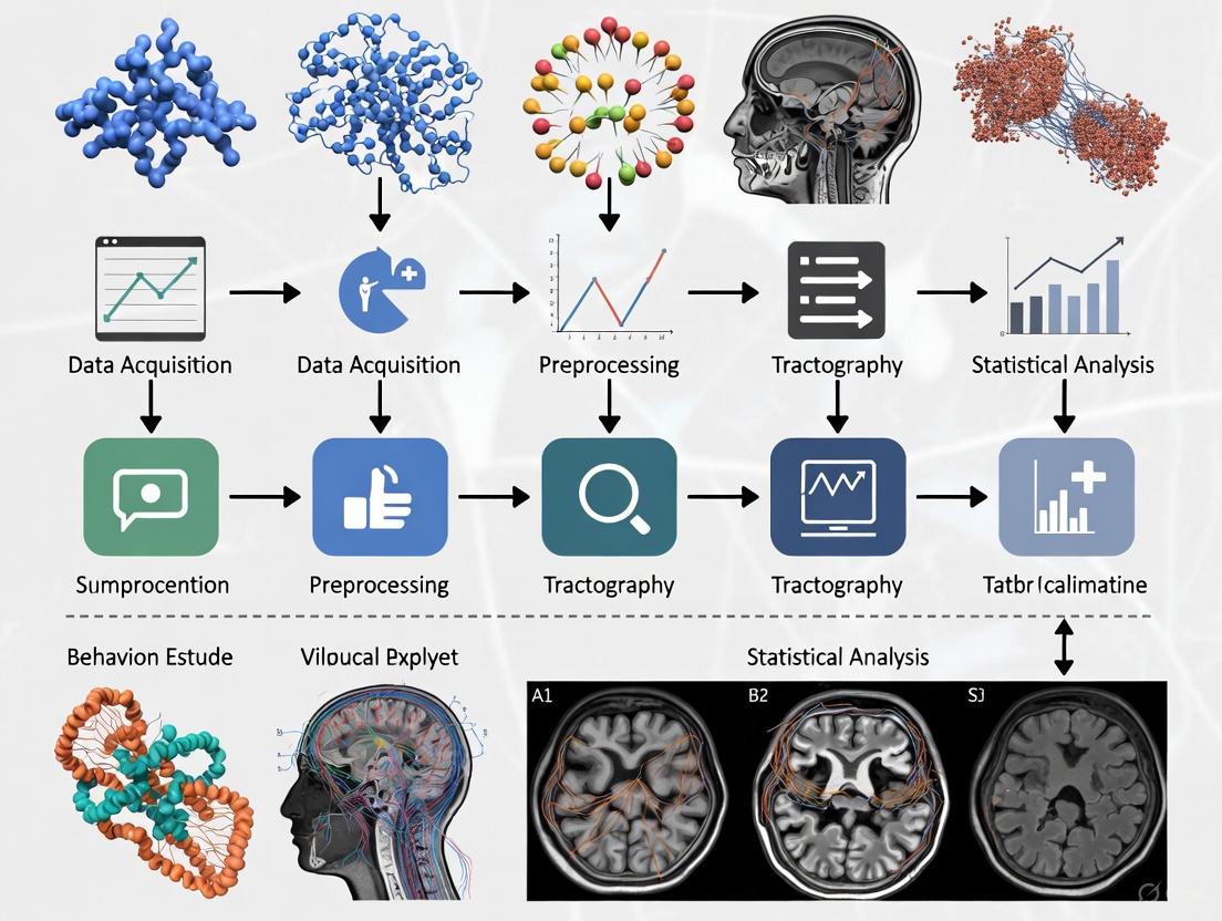
DTI Analysis Workflow

The diagram below outlines the standard workflow for processing and analyzing DTI data, from acquisition to statistical inference, which is crucial for managing large studies.

Research Reagent Solutions: Essential Tools for DTI Research

The following table details key software and methodological "reagents" essential for conducting DTI studies.

Tool / Method	Function	Relevance to Large Datasets
Riemannian Tensor Framework	Provides a robust mathematical foundation for tensor interpolation, averaging, and statistical calculation, using the full tensor information [4].	Enables more accurate population-level statistics and registration in large-scale studies by properly handling the tensor data structure [4].
Fiber Tract-Oriented Statistics	An object-oriented analysis approach where statistics are computed along specific fiber bundles rather than on a voxel-by-voxel basis [4].	Reduces data dimensionality and provides a more biologically meaningful analysis of white matter properties across a cohort [4].
ACT Rules & Accessibility Testing	A framework of rules for accessibility conformance testing, emphasizing the need for sufficient color contrast in visualizations [5].	Ensures that tractography visualizations and result figures are interpretable by all researchers, a key concern for collaboration and publication [5].

Advanced Troubleshooting & Artifact Handling

Frequently Asked Questions

We are seeing geometric distortions in our DTI data. What is the likely cause and solution? Geometric distortions and B0-susceptibility artifacts are common in EPI-based DTI, especially near tissue-air interfaces (e.g., the sinuses) [3]. This can be addressed by:

• Increasing the image bandwidth to reduce distortion at the cost of SNR.
• Using spin-echo (FSE) or line scan (LSDI) sequences instead of EPI, though these typically have longer acquisition times [3].
• Applying post-processing distortion correction algorithms, which often require acquiring data with reversed phase-encoding directions.

How can we ensure our DTI results are reproducible and comparable across different scanners? Scanner-specific protocols and hardware differences are a major challenge. To ensure reproducibility:

• Standardize your acquisition protocol (e.g., resolution, b-value, number of directions) across all sites in a multi-center study.
• Implement a "human phantom" phenomenon [1]. Scan a single subject on different scanners to establish a scaling factor, enabling comparison to normative databases acquired on different hardware [1].

What is the recommended color contrast for creating publication-quality diagrams and visualizations? For legibility, follow web accessibility guidelines (WCAG). Use a contrast ratio of at least 4.5:1 for normal text and 3:1 for large-scale text or user interface components against their background [6]. This ensures that all elements of your diagrams, such as text in nodes and the colors of arrows, are clearly distinguishable for all readers.

Core DTI Metrics Reference Tables

Primary Scalar Metrics from the Diffusion Tensor

Table 1: Key Scalar DTI Metrics Derived from Eigenvalues (λ₁, λ₂, λ₃)

Metric Name	Acronym	Formula	Biological Interpretation	Clinical & Research Context
Fractional Anisotropy	FA	( \textrm{FA} = \frac{\sqrt{(\lambda1 - \lambda)^2 + (\lambda2 - \lambda)^2 + (\lambda3 - \lambda)^2}}{\sqrt{\lambda1^2 + \lambda2^2 + \lambda3^2}} ) [7]	Degree of directional water diffusion restriction; reflects white matter "integrity" (axonal density, myelination, fiber coherence) [8].	Increase: Often associated with brain development [8]. Decrease: Linked to axonal damage, demyelination (e.g., TBI, MS, AD) [9] [8].
Mean Diffusivity	MD	( \textrm{MD} = \frac{\lambda1 + \lambda2 + \lambda_3}{3} ) [10]	Magnitude of average water diffusion, irrespective of direction [9].	Increase: Suggests loss of structural barriers, often seen in edema, necrosis, or neurodegeneration [11].
Axial Diffusivity	AD	( \textrm{AD} = \lambda_1 )	Diffusivity parallel to the primary axon direction.	Decrease: Interpreted as axonal injury [3].
Radial Diffusivity	RD	( \textrm{RD} = \frac{\lambda2 + \lambda3}{2} )	Average diffusivity perpendicular to the primary axon direction.	Increase: Interpreted as demyelination [3].

Advanced Diffusion Models

Table 2: Advanced Diffusion Metrics Beyond the Standard Tensor Model

Model/Metric	Acronym	Description	Interpretation & Advantage
Tensor Distribution Function	TDF	Probabilistic mixture of tensors to model multiple underlying fibers [11].	Overcomes single-tensor limitation in crossing-fiber regions; provides "corrected" FA (FATDF) shown to be more sensitive to disease effects (e.g., in Alzheimer's disease) [11].
Mean Kurtosis	MK	Quantifies the degree of non-Gaussian water diffusion [12].	Higher MK suggests greater microstructural complexity; sensitive to pathological changes in both gray and white matter [12].
Neurite Orientation Dispersion and Density Imaging	NODDI	Multi-compartment model separating intra-neurite, extra-neurite, and CSF signal [12].	Provides specific metrics like neurite density (NDI) and orientation dispersion (ODI), offering more biological specificity than DTI [12].
Generalized Fractional Anisotropy	GFA	An analog of FA for models like Q-Ball imaging, based on the orientation distribution function (ODF) [8].	Measures variation of the ODF; useful for high angular resolution diffusion imaging (HARDI) methods [8].

Troubleshooting Guides & FAQs

Data Quality & Metric Interpretation

Q1: Our study shows a statistically significant decrease in Fractional Anisotropy in a patient group. Can we directly conclude this indicates a loss of "white matter integrity"?

Not directly. While often interpreted as a marker of white matter integrity, a decrease in FA is not specific to a single biological cause [8]. It can result from:

• A decrease in Axial Diffusivity (suggesting axonal injury).
• An increase in Radial Diffusivity (suggesting demyelination) [8].
• Complex changes in both AD and RD.
• An increase in fiber crossing or dispersion not related to pathology [11].
• Recommendation: Always consult AD and RD metrics alongside FA to generate more specific hypotheses about the underlying microstructural change [3].

Q2: We are getting inconsistent FA values in brain regions with known crossing fibers. How can we improve accuracy?

This is a classic limitation of the single-tensor model, which can only represent one dominant fiber orientation per voxel [11].

• Solution: Employ advanced reconstruction models designed for complex fiber architecture, such as the Tensor Distribution Function (TDF) or Constrained Spherical Deconvolution (CSD) [11]. These models provide more accurate anisotropy estimates in regions with crossing, kissing, or fanning fibers.

Q3: Our multi-site DTI study shows high inter-scanner variability in metric values. How can we ensure data consistency?

This is a common challenge due to differences in scanner hardware, software, and gradient performance [13] [14].

• Solution: Implement a rigorous, phantom-based Quality Assurance (QA) protocol [13] [15] [12].
  • Use a stable, agar-filled diffusion phantom [15] [12].
  • Conduct regular scans of the phantom to track the scanner's performance over time.
  • Use automated QA tools (e.g., the publicly available qa-dti tool [15]) to extract metrics like SNR, eddy current-induced distortions, and FA uniformity [13] [15]. This allows you to quantify and correct for inter-site and inter-scanner differences.

Q4: What are the primary sources of artifacts in DTI data, and how can they be mitigated?

Table 3: Common DTI Artifacts and Correction Strategies

Artifact Type	Cause	Impact on DTI Metrics	Mitigation Strategies
Eddy Current Distortions	Rapid switching of strong diffusion-sensitizing gradients.	Geometric distortions in DWI images; inaccurate tensor estimation [3].	Use of "dual spin-echo" sequences [15]; post-processing correction tools (e.g., eddy in FSL) [13] [3].
EPI Distortions (B0 Inhomogeneity)	Magnetic field (B0) inhomogeneities, especially near sinuses.	Severe geometric stretching or compression [3].	Use of parallel imaging (SENSE, GRAPPA) to reduce echo train length [3]; B0 field mapping (e.g., with FUGUE) for post-processing correction [13].
Subject Motion	Head movement during the relatively long DTI acquisition.	Blurring, misalignment between diffusion volumes, corrupted tensor fitting [3].	Proper head stabilization; prospective motion correction; post-processing realignment and registration [3].
Systematic Spatial Errors	Nonlinearity of the magnetic field gradients.	Inaccurate absolute values of diffusion tensors, affecting cross-scanner comparability [14].	Use of the B-matrix Spatial Distribution (BSD-DTI) method to characterize and correct for gradient nonuniformities [14].

Experimental Protocol & Analysis

Q5: What is the minimum number of diffusion gradient directions required for a robust DTI study?

While more directions are always better, a common recommendation is a minimum of 20 diffusion directions, with 30 or more (e.g., 64) being preferred for robust tensor estimation and fiber tracking [10]. The exact number depends on the desired accuracy and the specific analysis (e.g., tractography requires more directions than a simple whole-brain FA analysis).

Q6: Our clinical scan time is limited. Can we still derive meaningful DTI metrics from a protocol with fewer gradient directions?

Yes. Research indicates that even with a reduced set of directions (e.g., 30, 15, or 7), meaningful group-level analyses are possible [11]. Furthermore, using advanced models like the Tensor Distribution Function (TDF) on such "clinical quality" data can yield FA metrics (FA_TDF) that are more sensitive to disease effects than standard FA from a full dataset, by better accounting for crossing fibers [11].

Detailed Experimental Protocols

Protocol 1: Phantom-Based DTI Quality Assurance

This protocol provides a methodology for monitoring scanner stability and ensuring data quality consistency, crucial for handling large multi-site or longitudinal datasets [13] [15] [12].

Objective: To establish a baseline and longitudinally track the performance of an MRI scanner for DTI acquisitions using an agar phantom.

Materials:

• Phantom: FBIRN-style agar-filled spherical phantom (stable, reproducible diffusion properties) [15].
• MRI Scanner: Equipped with a multi-channel head coil.

Acquisition Parameters:

• The DTI acquisition protocol (b-value, number of diffusion directions, phase encode steps) should match the parameters used for human subject scans to accurately assess performance.
• Repetition Time (TR) can be minimized as full brain coverage is not needed.
• A central slab (thick slice or average of a few slices) is acquired to ensure high SNR [15].

Processing & Analysis (Automated): The following workflow can be implemented using automated tools like the publicly available qa-dti code [15].

Key Outcome Metrics: The protocol generates eleven key metrics, including [13] [15]:

• SNR (nDWI and DWI): Measures signal stability and gradient performance.
• Shape Analysis (Sphericity): Quantifies distortions from eddy currents and B0 inhomogeneity.
• FA Value and Uniformity: Tracks the accuracy and consistency of the primary DTI metric in the phantom.
• Nyquist Ghosting: Assesses EPI-related artifacts.

Protocol 2: In-Vivo DTI Processing for Large Cohort Analysis

This protocol outlines a standardized pipeline for processing human DTI data, which is essential for ensuring reproducibility and validity in studies with large datasets.

Objective: To preprocess and reconstruct DTI data from human subjects for group-level statistical analysis.

Materials:

• Raw DWI Data: Including multiple b=0 s/mm² images (nDWI) and multiple diffusion-weighted images (DWI).
• Structural T1-weighted Image: For co-registration and anatomical reference.
• Software: Tools like FSL, DTIStudio, DTIprep, or TORTOISE [13] [3].

Processing & Analysis: The standard pipeline involves several critical steps to correct for common artifacts.

Critical Steps:

• Eddy Current & Motion Correction: Uses tools like eddy (FSL) to correct for distortions from gradient switching and subject head motion [13] [3].
• EPI Distortion Correction: Uses B0 field maps (e.g., with FUGUE) to correct for geometric distortions caused by magnetic field inhomogeneities [13] [3].
• Tensor Fitting & Metric Calculation: The diffusion tensor is fitted at each voxel to derive FA, MD, AD, and RD maps [3].
• Spatial Normalization & Group Analysis:
  • Tract-Based Spatial Statistics (TBSS): A highly recommended approach for voxel-wise group analysis. All subjects' FA data are aligned to a common space and projected onto a mean FA skeleton, which mitigates registration issues and avoids the need for arbitrary spatial smoothing [9]. This increases the sensitivity and reliability of statistical comparisons.

The Scientist's Toolkit

Table 4: Essential Research Reagents & Materials for DTI Studies

Item Name	Category	Function & Rationale
Agar Diffusion Phantom	Quality Assurance	Provides a stable, reproducible reference with known diffusion properties to monitor scanner performance, validate sequences, and ensure cross-site and longitudinal consistency [13] [12].
BSD-DTI Correction	Software/Algorithm	Corrects for spatial systematic errors in the diffusion tensor caused by gradient nonlinearities, improving the accuracy and comparability of absolute metric values, especially in multi-scanner studies [14].
Tract-Based Spatial Statistics (TBSS)	Analysis Software	A robust software pipeline within FSL for performing voxel-wise multi-subject statistics on FA and other diffusion metrics, minimizing registration problems and increasing statistical power [9].
Advanced Reconstruction Models (TDF, CSD, NODDI)	Software/Algorithm	Mathematical frameworks that overcome the limitations of the single-tensor model, providing more accurate metrics in complex white matter regions and potentially greater sensitivity to disease-specific changes [11] [12].
3-Ethyl-4-octanol	3-Ethyl-4-octanol, CAS:63126-48-7, MF:C10H22O, MW:158.28 g/mol	Chemical Reagent
3-Chloro-2-phenylprop-2-enamide	(E)-3-chloro-2-phenylprop-2-enamide|High-Purity Reference Standard	(E)-3-chloro-2-phenylprop-2-enamide (C9H8ClNO). A cinnamamide derivative for antimicrobial and anticonvulsant research. For Research Use Only. Not for human or veterinary use.

FAQs and Troubleshooting Guides

This section addresses common challenges researchers face when handling the "Three V's" of Big Data—Volume, Velocity, and Variety—in Diffusion Tensor Imaging (DTI) studies.

FAQ 1: How can we manage the massive Volume of raw DTI data?

• Challenge: Raw DTI data from large cohorts can consume terabytes of storage. For example, a dataset from just 10,000 individuals can require over 13.5 TB of space for NIfTI files alone [16]. This volume strains storage systems and complicates data backup.

• Solutions:

  • Utilize Processed Data: For specific questions, use preprocessed data (e.g., connectivity matrices), which can reduce storage needs to a fraction of the raw data size [16].
  • Cloud & Distributed Storage: Leverage cloud data warehouses (e.g., Snowflake, BigQuery) or distributed file systems (e.g., Hadoop HDFS) that offer scalable, virtually infinite storage [17] [18] [19].
  • Strategic Backups: When backing up data, consider excluding intermediate processed files that can be regenerated, focusing only on irreplaceable raw data [16].

• Troubleshooting Guide: "My research group is running out of storage space for our DTI datasets."

Step	Action	Rationale
1	Audit Data	Identify and archive raw data that is no longer actively needed for analysis.
2	Implement a Data Tiering Policy	Move older, infrequently accessed datasets to cheaper, long-term storage solutions.
3	Use Data Compression	Apply lossless compression to NIfTI files to reduce their footprint without losing information.
4	Consider Processed Data	If your research question allows, download only the preprocessed scalar maps (FA, MD) for analysis.

FAQ 2: How do we handle the Variety and inconsistency of DTI data from different sources or protocols?

• Challenge: DTI data can come in varied formats (DICOM, NIfTI), from different scanner manufacturers, and with different acquisition parameters (b-values, gradient directions). This inconsistency makes pooling data for large-scale studies difficult [18] [20] [19].

• Solutions:

  • Standardize with BIDS: Organize your data according to the Brain Imaging Data Structure (BIDS) standard. This ensures a consistent and predictable structure, making data easier to share, process, and understand [16].
  • Data Integration Tools: Use data integration tools to create reliable pipelines that can pull data from hundreds of different sources and apply transformations for consistency [17].
  • Detailed Documentation: Meticulously document all acquisition parameters, preprocessing steps, and software versions used for each dataset [16].

• Troubleshooting Guide: "I cannot combine my DTI dataset with a public dataset due to format and parameter differences."

Step	Action	Rationale
1	Convert to Standard Format	Ensure all datasets are in the same standard format, preferably NIfTI, using tools like dcm2niix [21].
2	Harmonize Acquisition Parameters	Note differences in b-values, number of gradient directions, and voxel size. Statistical harmonization methods (e.g., ComBat) may be required to adjust for these differences.
3	Spatial Normalization	Register all individual DTI maps (FA, MD) to a common template space (e.g., FMRIB58_FA) to enable voxel-wise group comparisons.
4	Use a Common Pipeline	Process all datasets through the same software pipeline (e.g., FSL's dtifit) to ensure derived metrics are comparable [21].

FAQ 3: What are the best practices for ensuring data Veracity (quality) in high-Velocity, automated DTI processing streams?

• Challenge: The push for faster (high-velocity) analysis and real-time insights increases the risk of propagating errors from poor-quality data. This includes artifacts from subject motion, eddy currents, and low signal-to-noise ratio [17] [3].

• Solutions:

  • Automated Quality Control (QC): Implement automated QC pipelines that quantify metrics like signal-to-noise ratio, motion parameters, and artifact detection for every dataset [16].
  • Data Observability: Go beyond simple monitoring. Use platforms that provide freshness, distribution, and lineage of your data to quickly identify and triage quality issues [17].
  • Visual Inspection: Never fully automate QC. Always include a step for manual visual inspection of raw data, intermediate steps, and final results to catch subtle errors automated systems might miss [16] [21].

• Troubleshooting Guide: "My automated DTI pipeline produced implausible tractography results for several subjects."

Step	Action	Rationale
1	Check Raw Data	Go back to the raw diffusion-weighted images. Look for severe motion artifacts, signal dropouts, or "zipper" artifacts that could corrupt the entire pipeline.
2	Inspect Intermediate Outputs	Check the outputs of key steps like eddy-current correction and brain extraction. A poorly generated brain mask can severely impact tensor fitting.
3	Review QC Metrics	Check the subject's motion parameters and outlier metrics from the eddy-current correction step. High values often explain poor results.
4	Re-run with Exclusions	For subjects with severe artifacts, consider excluding the affected volumes (if using a modern tool like FSL's eddy) or excluding the subject entirely.

Experimental Protocols for DTI Analysis

This section provides detailed methodologies for key experiments in DTI research, incorporating best practices for handling large datasets.

Protocol 1: Multi-Site DTI Analysis for Large-Scale Studies

This protocol is designed for pooling and analyzing DTI data collected across multiple scanners and sites, a common scenario in large-scale consortia studies like the UK Biobank or ABCD [16] [22].

• 1. Data Acquisition Harmonization:

  • Aim: Minimize site-related variability at the source.
  • Method:
    • Use standardized acquisition protocols across all sites where possible.
    • Employ phantom studies to quantify and correct for inter-scanner differences in DTI metrics.
    • Collect high-resolution structural scans (T1-weighted, T2-weighted) alongside DTI for registration and tissue segmentation [22].

• 2. Centralized Data Processing & Quality Control:

  • Aim: Ensure consistent and high-quality data processing for all subjects.
  • Method:
    • Storage: Use a centralized, cloud-based storage platform (e.g., a data lakehouse) to aggregate all datasets [17].
    • Preprocessing: Run all data through a single, version-controlled pipeline. Key steps include:
      • Denoising
      • Eddy-current and motion correction
      • Outlier volume rejection
      • Tensor fitting to create Fractional Anisotropy (FA) and Mean Diffusivity (MD) maps [21].
    • Quality Control: Implement an automated QC pipeline that flags datasets for excessive motion, artifacts, or poor registration. All flagged datasets must undergo manual inspection.

• 3. Statistical Analysis and Data Integration:

  • Aim: Derive meaningful insights from the harmonized dataset.
  • Method:
    • Voxel-Based Analysis (VBA): Non-linearly register all FA maps to a standard template. Perform voxel-wise cross-subject statistics to identify regions where DTI metrics correlate with clinical or demographic variables [4].
    • Tract-Based Spatial Statistics (TBSS): Project all FA data onto a mean FA skeleton before performing statistics, which reduces alignment issues and is considered more robust than VBA.
    • Data Integration: Link DTI metrics with phenotypic, genetic, or behavioral data stored in a structured format (e.g., SQL database) for multivariate analysis [16].

The workflow for this protocol can be visualized as follows:

Protocol 2: Accelerated DTI Acquisition and Reconstruction using Deep Learning

This protocol addresses the Velocity challenge by reducing scan times, which is critical for clinical practice and large-scale studies [23] [22].

• 1. Data Acquisition for Model Training:

  • Aim: Acquire a high-quality reference dataset for training a deep learning model.
  • Method:
    • Acquire DTI data with a high number of gradient directions (e.g., 60-90 directions) and multiple b=0 volumes to serve as the ground truth [22].
    • Include high-resolution T1-weighted and T2-weighted structural images to provide complementary spatial information [23].

• 2. Model Training for Image Synthesis:

  • Aim: Train a model to predict high-quality DWI volumes from a highly undersampled acquisition.
  • Method:
    • Framework: Use a deep learning framework like DeepDTI [23].
    • Input: The model takes as input a minimal set of data—one b=0 and six diffusion-weighted images (DWIs) along with structural T1 and T2 volumes.
    • Output: The model is trained to output the residuals between the input low-quality images and the target high-quality DWI volumes.
    • Architecture: A 3D Convolutional Neural Network (CNN) is used to leverage redundancy in local, non-local, and cross-contrast spatial information [23].

• 3. Validation and Tractography:

  • Aim: Ensure the accelerated method produces biologically valid results.
  • Method:
    • Tensor Fitting: Fit the diffusion tensor to the model's output high-quality DWIs to generate standard scalar maps (FA, MD) and the primary eigenvector map [23] [21].
    • Validation: Quantitatively compare the DeepDTI-derived metrics and resulting tractography against the ground truth from the fully sampled data. Metrics like mean distance between reconstructed tracts should be used (e.g., target: 1-1.5 mm) [23].

The following diagram illustrates the core DeepDTI processing framework:

The Scientist's Toolkit: Research Reagent Solutions

The following table details essential software, data, and hardware "reagents" required for modern DTI research involving large datasets.

Research Reagent	Type	Function / Application
FSL (FDT, BET, dtifit) [21]	Software Library	A comprehensive suite for DTI preprocessing, tensor fitting, and tractography. Essential for creating standardized analysis pipelines.
Brain Imaging Data Structure (BIDS) [16]	Data Standard	A standardized framework for organizing neuroimaging data. Critical for ensuring data reproducibility, shareability, and ease of use in large-scale studies.
Cloud Data Platforms (e.g., Snowflake, BigQuery) [17]	Data Infrastructure	Provide scalable storage and massive parallel processing capabilities for handling the Volume of large DTI datasets and associated phenotypic information.
High-Field MRI Scanner (5.0T-7.0T) [22]	Hardware	Provides higher spatial resolution and Signal-to-Noise Ratio (SNR) for DTI, improving the accuracy of tractography and microstructural measurements.
Deep Learning Models (e.g., DeepDTI) [23]	Software Algorithm	Enables significant acceleration of DTI acquisition by synthesizing high-quality data from undersampled inputs, directly addressing the Velocity challenge.
Large-Scale Open Datasets (e.g., HCP, UK Biobank, Diff5T) [16] [22]	Data Resource	Provide pre-collected, high-quality data from thousands of subjects, enabling studies with high statistical power and the development of normative atlases.
Data Observability Platform (e.g., Monte Carlo) [17]	Data Quality Tool	Monitors data pipelines for freshness, schema changes, and lineage, helping to maintain Veracity across large, complex data ecosystems.
N-benzyl-5,5-dimethyloxolan-3-amine	N-benzyl-5,5-dimethyloxolan-3-amine|CAS 1935643-50-7	High-purity N-benzyl-5,5-dimethyloxolan-3-amine (C13H19NO) for pharmaceutical and organic synthesis research. For Research Use Only. Not for human or veterinary use.
(1R)-1-Cyclopropylprop-2-yn-1-ol	(1R)-1-Cyclopropylprop-2-yn-1-ol, CAS:1867621-64-4, MF:C6H8O, MW:96.129	Chemical Reagent

Clinical and Research Applications in Behavioral Neuroscience

Troubleshooting Guide: DTI in Behavioral Neuroscience

Common DTI Data Quality Issues and Solutions

Problem Symptom	Potential Cause	Diagnostic Steps	Solution
Low Signal-to-Noise Ratio (SNR) [1] [24]	Short scan time, high b-value, long echo time (TE), hardware limitations [25].	Check mean diffusivity maps for unexpected noise; calculate tSNR in a homogeneous white matter region [25].	Increase number of excitations (NEX); use denoising algorithms (e.g., Marchenko-Pastur PCA) [25]; reduce TE if possible [25].
Image Distortion (Eddy Currents) [24]	Rapid switching of strong diffusion gradients [24].	Visual inspection of raw DWI for shearing or stretching artifacts [24].	Use pulsed gradient spin-echo sequences; apply post-processing correction (e.g., FSL's EDDY) [25].
Motion Artifacts [24]	Subject movement during scan [24].	Check output from motion correction tools (e.g., EDDY) for excessive translation/rotation [25].	Improve subject head stabilization; use faster acquisition sequences (e.g., single-shot EPI); apply motion correction [24].
Coregistration Errors	Misalignment between DTI slices or with anatomical scans.	Visual inspection of registered images for blurring or misaligned edges.	Ensure use of high-quality b=0 image for registration; align DWI to first TE session; check and rotate b-vectors [25].
Abnormal FA/MD Values	Pathological finding, or partial volume effect from CSF.	Correlate with T2-weighted anatomical images; check if values are consistent across nearby slices.	Use more complex models (e.g., NODDI) for specific microstructural properties [25]; ensure proper skull stripping [24].

Frequently Asked Questions (FAQs)

Q1: Our deep learning model for classifying CSM severity is overfitting. What strategies can we use? A1: Consider using a pre-trained network and freezing its parameters to prevent overfitting [26]. Implement a feature fusion mechanism, like DCSANet-MD, which integrates both 2D (maximally compressed disc) and 3D (whole spinal cord) features to provide a larger, more robust decision framework [26]. Data augmentation techniques specific to DTI can also be beneficial.

Q2: How does the choice of Echo Time (TE) impact DTI metrics, and how should we account for it? A2: DTI metrics are TE-dependent [25]. Increases in TE can lead to decreased Fractional Anisotropy (FA) and Axial Diffusivity (AD), and increased Mean Diffusivity (MD) and Radial Diffusivity (RD) [25]. For consistent results, use a fixed TE across all subjects in a study. If comparing across studies, the TE parameter must be considered. Multi-echo DTI acquisitions can help disentangle these effects [25].

Q3: What is the best way to define Regions of Interest (ROIs) for analysis to minimize subjectivity? A3: Manual ROI drawing is susceptible to human expertise and can yield inconsistent outcomes [26]. To minimize subjectivity, consider using standardized atlases (e.g., JHU white matter atlas) [25] or automated, deep-learning-based methods that perform end-to-end analysis without manual intervention [26].

Q4: We have a large, multi-session DTI dataset. What is a robust preprocessing pipeline? A4: A standard pipeline includes: 1) Denoising (e.g., using dwidenoise in MRtrix3) [25]; 2) B0-inhomogeneity correction (e.g., FSL's TOPUP) [25]; 3) Eddy current and motion correction (e.g., FSL's EDDY) [25]; 4) Brain extraction (skull stripping); and 5) Co-registration of all images to a common space [24].

Q5: How can we validate the quality of our acquired DTI dataset? A5: Perform both visual inspection and quantitative checks [25]. Visually check for ghosting or distortions in the mean DWIs [25]. Quantitatively, calculate the temporal Signal-to-Noise Ratio (tSNR) and monitor head motion parameters (translation, rotation) provided by tools like EDDY [25].

DTI Quantitative Metrics and Experimental Parameters

Key DTI Scalar Metrics

Metric	Full Name	Biological Interpretation	Typical Use Case in Behavioral Neuroscience
FA	Fractional Anisotropy [1]	Degree of directional water diffusion; reflects white matter integrity/organization [1].	Correlating WM integrity with cognitive scores (e.g., JOA score in CSM) [26].
MD / ADC	Mean Diffusivity / Apparent Diffusion Coefficient [1] [24]	Overall magnitude of water diffusion; increases can indicate edema or necrosis [1].	Detecting general tissue changes in neurodegenerative diseases [24].
AD	Axial Diffusivity [1]	Diffusion rate parallel to the main axon direction; may indicate axonal integrity [1].	Differentiating specific types of axonal injury in trauma models [24].
RD	Radial Diffusivity [1]	Diffusion rate perpendicular to the axon; may reflect myelin integrity [1].	Assessing demyelination in disorders like multiple sclerosis [24].

Example Experimental Protocol for CSM Severity Classification

Objective: To automatically classify the severity of Cervical Spondylotic Myelopathy (CSM) using deep learning on DTI data [26].

Dataset:

• Subjects: 176 CSM patients (112 male, 64 female, mean age 63.8 ± 13.7 years) [26].
• Clinical Ground Truth: Japanese Orthopaedic Association (JOA) score [26].
• Severity Categorization (Example):
  • Binary: Severe (JOA ≤ 9), Mild (JOA ≥ 10) [26].
  • Three-class: Severe (JOA ≤ 9), Moderate (JOA 10-12), Mild (JOA ≥ 13) [26].

DTI Acquisition (Example from cited research):

• Scanner: 3T Philips Achieva [26].
• Sequence: Single-shot Echo Planar Imaging (EPI) [26].
• Parameters: b-value = 600 s/mm², 15 directions, NEX=3, 12 slices covering C2-C7 [26].

Preprocessing:

• Feature Calculation: Use Spinal Cord Toolbox to calculate Fractional Anisotropy (FA) maps [26].
• Spatial Feature Selection: Extract the DTI slice at the Maximally Compressed Cervical Disc (MCCD) and the 3D DTI scan of the entire spinal cord [26].

Model & Analysis:

• Model: DCSANet-MD (DTI-Based CSM Severity Assessment Network-Multi-Dimensional) [26].
• Architecture: Employs two parallel residual networks (DCSANet-2D and DCSANet-3D) to extract features from the 2D MCCD slice and the 3D whole-cord scan, followed by a feature fusion mechanism [26].
• Results: The model achieved 82% accuracy in binary classification (mild vs. severe) and ~68% accuracy in the three-category classification [26].

DTI Analysis Workflow

The Scientist's Toolkit: Essential DTI Research Reagents & Solutions

Item Name	Function / Role	Example Usage / Notes
Diffusion-Weighted Images (DWI)	Raw data input; images sensitive to water molecule diffusion in tissues [24].	Acquired with multiple gradient directions and b-values to probe tissue microstructure [25].
Fractional Anisotropy (FA) Map	Primary computed metric; quantifies directional preference of water diffusion [1].	Used as the key input feature for deep learning models assessing white matter integrity [26].
Spinal Cord Toolbox (SCT)	Software for processing and extracting metrics from spinal cord MRI data [26].	Used for automated extraction of DTI features like FA maps from the cervical spinal cord [26].
FSL (FMRIB Software Library)	Comprehensive brain MRI analysis toolbox, includes DTI utilities [25].	Used for EDDY (correction for eddy currents and motion) and DTIFIT (tensor fitting) [25].
Deep Learning Framework (e.g., PyTorch, TensorFlow)	Platform for building and training custom neural network models [26].	Used to implement architectures like DCSANet-MD for automated classification tasks [26].
JHU White Matter Atlas	Standardized atlas defining white matter tract regions [25].	Used for ROI-based analysis to ensure consistent and comparable regional measurements across studies [25].
4-hydroxy-N,N-dimethylbutanamide	4-Hydroxy-N,N-dimethylbutanamide|CAS 18190-25-5	4-Hydroxy-N,N-dimethylbutanamide (CAS 18190-25-5). A biochemical building block for peptide synthesis and research. For Research Use Only. Not for human use.
3-Fluoro-4-nitrobenzaldehyde oxime	3-Fluoro-4-nitrobenzaldehyde Oxime|Research Use Only	3-Fluoro-4-nitrobenzaldehyde oxime for scientific research. Explore its applications in organic synthesis and as a biochemical building block. For Research Use Only. Not for human or veterinary use.

White Matter Architecture and Microstructural Correlates

Troubleshooting Guides & FAQs

This technical support resource addresses common challenges in diffusion MRI (dMRI) research, particularly within the context of managing large-scale datasets for behavioral studies.

Data Quality & Preprocessing

Q: Our diffusion measures (e.g., FA, MD) show unexpected variations between study sites in a multicenter trial. What could be the cause and how can we mitigate it?

A: Variations in dMRI data quality are a major confounder in multicenter studies. Key data quality metrics, including contrast-to-noise ratio (CNR), outlier slices, and participant motion (both relative and rotational), often differ significantly between scanning centers. These factors have a widespread impact on core diffusion measures like Fractional Anisotropy (FA) and Mean Diffusivity (MD), as well as tractography outcomes, and this impact can vary across different white matter tracts. Notably, these effects can persist even after applying data harmonization algorithms [27].

• Mitigation Strategy: Always include data quality metrics as covariates in your statistical models. This is critical for analyzing individual differences or group effects in multisite datasets. Proactively monitoring these metrics during data acquisition can also help identify and rectify issues early [27].

Q: How can we handle the confounding effects of age when studying a clinical population across a wide age range?

A: Age-related microstructural changes are a pervasive factor in white matter architecture. Conventional DTI metrics follow well-established trajectories: FA typically shows a non-linear inverted-U pattern across the lifespan, while MD, Axial Diffusivity (AD), and Radial Diffusivity (RD) generally increase with older age, reflecting declining microstructural integrity [28]. Advanced dMRI models (e.g., NODDI, RSI) can provide additional sensitive measures to age-related changes [28].

• Mitigation Strategy: For cross-sectional studies, carefully age- and sex-match your patient and control groups. In longitudinal studies or those with wide age ranges, use statistical methods like linear mixed effects models to explicitly model and account for age trajectories [28] [29].

Experimental Design & Interpretation

Q: We are observing higher Fractional Anisotropy (FA) in early-stage patient groups compared to controls, which contradicts the neurodegenerative disease hypothesis. Is this plausible?

A: Yes, this seemingly paradoxical finding is biologically plausible and has been documented. A large worldwide study of Parkinson's disease (PD) found that in the earliest disease stage (Hoehn and Yahr Stage 1), participants displayed significantly higher FA and lower MD across much of the white matter compared to controls. This is interpreted as a potential early compensatory mechanism, which is later overridden by degenerative changes (lower FA, higher MD) in advanced stages [29]. Similar considerations may apply to other disorders.

• Recommendation: Do not dismiss findings of increased FA out of hand. Interpret your results within the context of disease stage. Early, hyper-compensatory phases may exist for some conditions, and analyzing a cohort that mixes early and late-stage patients could obscure these distinct biological signatures [29].

Q: What is the justification for averaging measures across homologous tracts (e.g., left and right) in a group analysis?

A: While a common practice, it should be done with caution. Research shows that while many of the strongest microstructural correlations exist between homologous tracts in opposite hemispheres, the degree of this coupling varies widely. Furthermore, many white matter tracts exhibit known hemispheric asymmetries [30]. Blindly averaging can mask these biologically meaningful lateralized differences.

• Recommendation: Initially, analyze left and right hemisphere tracts separately to check for asymmetries or lateralized effects. Averaging is only justified if your statistical analysis confirms no significant hemispheric differences or interactions for your specific research question [30].

Summarized Quantitative Data

Table 1: Representative Microstructural Alterations Across Parkinson's Disease Stages

Data adapted from a worldwide study of 1,654 PD participants and 885 controls, comparing against matched controls [29].

Hoehn & Yahr Stage	Fractional Anisotropy (FA) Profile (vs. Controls)	Key Implicated White Matter Regions	Effect Size Range (Cohen's d)
Stage 1	Significantly higher FA	Anterior corona radiata, Anterior limb of internal capsule	d = 0.23 to 0.24
Stage 2	Lower FA in specific tracts	Fornix	d = -0.27
Stage 3	Lower FA in more regions	Fornix, Sagittal stratum	d = -0.29 to -0.31
Stage 4/5	Widespread, significantly lower FA	Fornix (most affected), 18 other ROIs	d = -0.38 to -1.09

Table 2: Common dMRI Data Quality Metrics and Their Impact

Based on an analysis of 691 participants (5-17 years) from six centers [27].

Data Quality Metric	Description	Impact on Diffusion Measures
Contrast-to-Noise Ratio (CNR)	Signal quality relative to noise	Low CNR can bias FA and MD values, reducing reliability.
Outlier Slices	Slices with signal drop-outs or artifacts	Can disrupt tractography, causing erroneous tract breaks or spurious connections.
Relative Motion	Subject movement relative to scan	Introduces spurious changes in diffusivity measures and reduces anatomical accuracy.
Rotational Motion	Rotational head movement during scan	Particularly detrimental to directional accuracy and anisotropy calculations.

Detailed Experimental Protocols

Protocol 1: Standardized DTI Tractography for Tract-Based Microstructural Analysis

This protocol is adapted from a foundational study investigating microstructural correlations across white matter tracts in 44 healthy adults [30].

• MRI Acquisition: Data were acquired on a 3T MRI scanner using a single-shot spin-echo EPI sequence.
  • Key Parameters: TE/TR = 63 ms/14 s, 55 diffusion-encoding directions at b=1000 s/mm², 1.8 mm isotropic voxels, 128x128 matrix [30].
• DTI Processing:
  • Brain Extraction: Remove non-brain tissue using a tool like FSL's BET [30].
  • Correction: Correct for eddy currents and subject motion using linear registration (e.g., FSL's FLIRT) of all diffusion-weighted images to the b=0 volume [30].
  • Tensor Fitting: Fit the diffusion tensor model in each voxel to compute maps of FA, MD, AD, and RD using software such as DTIstudio or FSL [30].
• Fiber Tractography:
  • Algorithm: Use deterministic Fiber Assignment by Continuous Tracking (FACT).
  • Parameters: Seed from all voxels with FA > 0.3. Continue tracking while FA > 0.2 and the turning angle between voxels is < 50° [30].
  • Tract Segmentation: Manually place Regions of Interest (ROIs) on directionally encoded color FA maps to isolate specific white matter tracts (e.g., Arcuate Fasciculus, Corticospinal Tract). Use exclusion ROIs to remove anatomically implausible fibers [30].
• Quantification: Extract mean FA, MD, AD, and RD values along the entire 3D trajectory of each reconstructed tract for statistical analysis [30].

Protocol 2: Quality Control and Harmonization for Multicenter dMRI Studies

This protocol outlines steps to manage data variability in large-scale, multi-scanner datasets [27].

• Proactive Harmonization: Standardize acquisition protocols across all sites whenever possible, including scanner manufacturer, model, field strength, and sequence parameters (b-values, number of directions, voxel size) [27].
• Quality Metric Extraction: For each dataset, compute a standard set of quality metrics:
  • Contrast-to-Noise Ratio (CNR)
  • Number of Outlier Slices
  • Motion Parameters (absolute, relative, translation, rotation) [27].
• Data Processing with Quality in Mind: Use modern pipelines (e.g., FSL, ANTs, MRtrix3) that include steps for denoising, eddy-current correction, and EPI distortion correction. Ensure gradient tables are correctly oriented after motion correction [31].
• Statistical Modeling: Include the extracted data quality metrics (Step 2) as nuisance covariates in all between-group or correlation analyses to statistically control for their influence [27].

Experimental Workflow Visualization

Diagram 1: Multicenter dMRI Data Analysis Workflow

Diagram 2: dMRI Preprocessing and Tractography Pipeline

The Scientist's Toolkit: Research Reagent Solutions

Table 3: Essential Software Tools for dMRI Analysis

Tool Name	Primary Function	Brief Description of Role
FSL (FMRIB Software Library)	Data Preprocessing & Analysis	A comprehensive library for MRI brain analysis. Its tools, like eddy_correct and FLIRT, are industry standards for correcting distortions and motion in dMRI data [30] [31].
DTIstudio / DSIstudio	Tractography & Visualization	Specialized software for performing deterministic fiber tracking and for the interactive selection and quantification of white matter tracts via ROIs [30].
MRtrix3	Advanced Tractography & Processing	Provides state-of-the-art tools for dMRI processing, including denoising, advanced spherical deconvolution-based tractography, and connectivity analysis [31].
ANTs (Advanced Normalization Tools)	Image Registration	A powerful tool for sophisticated image registration, often used for EPI distortion correction by non-linearly aligning dMRI data to structural T1-weighted images [31].
ENIGMA-DTI Protocol	Standardized Analysis	A harmonized pipeline for skeletonized TBSS analysis, enabling large-scale, multi-site meta- and mega-analyses of DTI data across research groups worldwide [29].
2-(Thiophen-2-yl)propanenitrile	2-(Thiophen-2-yl)propanenitrile CAS 88701-59-1
Ethyl 2-(3-ethoxyoxan-4-yl)acetate	Ethyl 2-(3-ethoxyoxan-4-yl)acetate|C11H20O4

DTI Acquisition Protocols and Computational Analysis Methods

Frequently Asked Questions (FAQs)

What is the b-value and how does it affect my diffusion MRI data?

The b-value (measured in s/mm²) is a factor that reflects the strength and timing of the gradients used to generate diffusion-weighted images (DWI) [32]. It controls the degree of diffusion-weighted contrast in your images, similar to how TE controls T2-weighting [32].

The signal in a DWI follows the equation: S = So * e^(–b • ADC), where So is the baseline MR signal without diffusion weighting, and ADC is the apparent diffusion coefficient [32]. A higher b-value leads to stronger diffusion effects and greater signal attenuation but also reduces the signal-to-noise ratio (SNR) [32] [33]. Choosing the correct b-value is crucial, as it directly impacts the quality of your derived quantitative measures, such as ADC maps, which are essential for analyzing large datasets in behavioral studies [33].

What is the recommended range of b-values for clinical and research studies?

The optimal b-value depends on the anatomical region, field strength, and predicted pathology [32]. The following table summarizes expert recommendations:

Table 1: Recommended b-value Ranges

Anatomical Region	Recommended b-value range (s/mm²)	Key Considerations
Brain (Adult)	0 – 1000 [33]	A useful rule of thumb is to pick the b-value so that (b × ADC) ≈ 1 [32].
Body	50 – 800 [33]	Includes areas like the liver and kidneys.
Neonates/Infants	600 – 700 [32]	Higher water content and longer ADC values require adjustment.
High-Contrast Microstructure	2000 – 3000 [33]	Provides specific information on tissue microstructure but with increased noise [32].

How many gradient directions should I use and why does it matter?

The number of diffusion gradient directions is critical for accurately modeling tissue anisotropy, especially in structured tissues like brain white matter.

Table 2: Guidelines for Gradient Directions

Application / Goal	Minimum Number of Directions	Rationale and Notes
Basic ADC calculation	3–4 directions [33]	Mitigates slight tissue anisotropy effects.
Full Diffusion Tensor Imaging (DTI)	≥ 6 non-collinear directions [33]	Required to calculate fractional anisotropy (FA) and tensor orientation in anisotropic tissues [33].
Multi-shell acquisitions	Different directions per shell [34]	Using the same directions for different b-value shells (e.g., b=1000 and b=2000) is not optimal. A multishell scheme with uniform coverage across all shells is a better approach [34].

What are the common artifacts and how can I correct for b-value inaccuracies?

Several artifacts can affect DWI data quality in large-scale studies:

• Geometric Distortions: Caused by magnetic susceptibility variations, especially at air-tissue interfaces [33].
• Eddy Currents: Induced by strong diffusion gradients, leading to image distortions [33].
• Gradient Deviations: The actual played-out b-value can deviate from its nominal value due to gradient nonlinearities, miscalibration, and other system imperfections [35]. This can lead to erroneous ADC and FA values.

An image-based method for voxel-wise b-value correction has been proposed to address these inaccuracies comprehensively [35]. The protocol involves:

• Phantom Scanning: Acquire DWI data (e.g., 64 directions) from a large isotropic water phantom at the target b-value (e.g., b=1000 s/mm²) [35].
• Calculate True ADC: Measure the phantom's temperature to determine the true diffusion constant of water (D_true) [35].
• Compute Correction Map: For each voxel and direction, compute a correction factor c = ADC_err / ADC_true, where ADC_err is the ADC calculated using the nominal b-value. The effective b-value is then b_eff = c * b_nom [35].
• Apply Correction: Use the calculated b_eff map to correct research or clinical DTI datasets, improving the accuracy of diffusivity and anisotropy measures [35].

Experimental Protocols

Protocol 1: Basic DWI Acquisition for ADC Mapping

This protocol is suitable for initial experiments focusing on general diffusion characterization.

• Pulse Sequence: Use a single-shot spin-echo Echo-Planar Imaging (EPI) sequence for its speed and robustness to motion [33].
• Parameter Optimization:
  • Repetition Time (TR): Use long TR (≥ 4500 ms) to minimize T1-weighting and maximize SNR [33].
  • Echo Time (TE): Use the minimum TE possible for the highest targeted b-value to reduce T2-decay and maximize SNR [33].
• b-values: Acquire at least two b-values: a low b-value (b=0 s/mm² or b=50 s/mm² for body) and a high b-value (e.g., b=800 or 1000 s/mm²) [33].
• Gradient Directions: A minimum of 3–4 directions is sufficient for a rotationally invariant ADC estimate in relatively isotropic tissues [33].
• Data Output: The raw data will consist of DICOM files for each b-value and direction. These must be processed (motion-corrected, etc.) before voxel-wise ADC calculation using the equation: ADC = ln(S_low / S_high) / (b_high - b_low) [36] [35].

Protocol 2: Comprehensive DTI for White Matter Tractography

This advanced protocol is designed for studies investigating white matter microstructure and connectivity in large datasets.

• Pulse Sequence: Single-shot spin-echo EPI, ideally with parallel imaging (e.g., SENSE, GRAPPA) to reduce TE and distortions [33].
• Parameter Optimization:
  • b-values: Acquire one b=0 volume and multiple b-values (e.g., b=1000 s/mm²) along many directions [33].
  • Averaging: To compensate for SNR loss at high b-values, increase the number of averages (NA) proportionally to the square root of the b-value [33].
• Gradient Directions: For a full diffusion tensor model, acquire at least 6 non-collinear directions for a single shell, though more directions (e.g., 30-64) are recommended for robust tensor estimation and tractography [34] [33].
• Data Output: The dataset will include multiple DWI volumes. Preprocessing for large studies should include correction for motion, eddy currents, and susceptibility distortions [37]. The output is a 4D data file ready for tensor fitting to generate FA, MD, and eigenvector maps.

Workflow Visualization

The following diagram illustrates the key decision points and steps for optimizing b-values and gradient directions in a diffusion MRI study.

The Scientist's Toolkit: Essential Research Reagents & Materials

Table 3: Key Materials for Diffusion MRI Quality Assurance

Item	Function in Experiment
Isotropic Water Phantom	A crucial tool for validating scanner performance, calibrating gradients, and measuring voxel-wise b-value maps. Its known diffusion properties provide a ground truth reference [38] [35].
Temperature Probe	Used to measure the temperature of the water phantom. This is essential for accurately determining the phantom's true diffusion coefficient (D_true), which is temperature-dependent [38] [35].
Geometric Distortion Phantom	A phantom with a known grid structure to quantify and correct for EPI-related geometric distortions in the acquired diffusion images [33].
B-value Correction Software	Custom or open-source scripts (e.g., in MATLAB) to implement voxel-wise correction algorithms, improving the accuracy of ADC and DTI metrics in large datasets [36] [35].
Diffusion Data Preprocessing Pipelines	Integrated software tools (e.g., FSL, DSI Studio) that perform critical steps like eddy current correction, motion artifact removal, and outlier rejection, which are essential for ensuring data quality in behavioral studies [37] [34].
1-(3-Chloro-2-methylphenyl)ethanol	1-(3-Chloro-2-methylphenyl)ethanol|C9H11ClO|RUO
(S)-alpha-benzhydryl-proline-HCl	(S)-alpha-benzhydryl-proline-HCl|CAS 1217653-75-2

Balancing Angular Resolution with Acquisition Time

In diffusion MRI research, particularly in studies involving large datasets for behavioral or drug development purposes, one of the most fundamental challenges is balancing the need for high angular resolution with the practical constraints of acquisition time. Higher angular resolution—achieved by acquiring more diffusion gradient directions—provides a more detailed characterization of complex white matter architecture, such as crossing fibers. However, this comes at the cost of longer scan times, which can increase susceptibility to patient motion, reduce clinical feasibility, and complicate the management of large-scale datasets. This guide provides targeted troubleshooting and FAQs to help researchers optimize this critical trade-off in their experimental protocols.

FAQs: Resolving Common Experimental Issues

1. How many diffusion gradient directions are sufficient for a reliable DTI study?

The optimal number of gradients is a balance between signal-to-noise ratio (SNR), accuracy, and time. While only six directions are mathematically required to fit a diffusion tensor, research studies require more for robustness.

• Evidence-Based Recommendations: A study scanning 50 healthy adults at 4 Tesla found that the SNR for common metrics like Fractional Anisotropy (FA) and Mean Diffusivity (MD) peaked at around 60-66 gradients [39]. Beyond this, adding more directions provided diminishing returns for these particular metrics. For studies aiming to reconstruct more complex fiber orientation distributions, accuracy may continue to improve with more gradients [39].
• Protocol Selection: The takeaway is that for standard DTI metrics, protocols with approximately 60 directions offer a good balance. For studies specifically focused on crossing fibers, a higher number may be warranted if acquisition time allows.

2. Should I prioritize higher spatial resolution or higher angular resolution when scan time is fixed?

This is a classic trade-off. In a fixed scan time, increasing the number of gradients (angular resolution) requires larger voxel sizes (lower spatial resolution) to maintain SNR, and vice-versa.

• The Trade-off: Studies comparing time-matched protocols have shown that protocols with larger voxels and higher angular resolution generally provide better SNR and improved stability of diffusion measures over time [40]. However, larger voxels increase partial volume effects, potentially biasing anisotropy measures [40].
• Guidance for Different Goals:
  • For tractography in regions with complex fiber crossings (e.g., kissing or crossing fibers), a high angular resolution is more critical [41].
  • For accurately distinguishing between closely neighboring anatomical structures (e.g., kissing fibers), a high spatial resolution is more beneficial [41].
  • Using "beyond-tensor" models can help mitigate the partial volume biases introduced by larger voxels [40].

3. My clinical DWI data has only 6 directions. Can I still use it for research?

While challenging, deep learning methods are being developed to enhance the utility of such limited data. One proposed method, DirGeo-DTI, uses directional encoding and geometric constraints to estimate reliable DTI metrics from as few as six directions, making retrospective studies on clinical datasets more feasible [42]. However, the performance of such models depends on the quality and diversity of their training data.

4. What are the most common pitfalls that affect DTI metric accuracy, beyond the number of directions?

The accuracy of your results can be compromised by multiple factors throughout the processing pipeline. Key pitfalls include [43]:

• Systematic Spatial Errors: Caused by inhomogeneities in the scanner's magnetic field gradients, these errors can significantly distort diffusion metrics. Correction methods like the B-matrix Spatial Distribution (BSD) are essential for accuracy [14] [44].
• Random Noise: Denoising techniques should be applied to the data. Combining denoising with BSD correction has been shown to significantly improve the quality of both DTI metrics and tractography [44].
• Subject Motion and Physiological Effects: Even with high gradient numbers, real-world factors like motion can limit the achievable SNR, making robust correction algorithms a necessity [39].

Troubleshooting Guides

Issue: Inconsistent or Noisy DTI Metrics Across Study Participants

Possible Causes and Solutions:

• Cause 1: Inadequate SNR due to an insufficient number of gradient directions or overly small voxels.
  • Solution: If increasing gradients is not feasible, consider increasing voxel size slightly or using a denoising algorithm as a preprocessing step [44] [40].
• Cause 2: Uncorrected systematic spatial errors from gradient non-uniformity.
  • Solution: Implement a correction method for the spatial distribution of the B-matrix (BSD-DTI) if available for your scanner and processing pipeline [14] [44].
• Cause 3: Failure of the tensor model in brain regions with complex fiber architecture (e.g., ~40% of white matter).
  • Solution: For studies focused on such regions, consider adopting a High Angular Resolution Diffusion Imaging (HARDI) technique that does not rely on a single tensor model, such as Q-ball imaging or spherical deconvolution [39] [41].

Issue: Tractography Fails to Resolve Crossing Fiber Pathways

Possible Causes and Solutions:

• Cause: The angular resolution of the acquisition is too low to accurately represent multiple fiber orientations within a single voxel.
  • Solution: Prioritize angular resolution over spatial resolution for this specific goal. Research indicates that for resolving crossings, high angular resolution is crucial, whereas high spatial resolution is better for distinguishing between kissing fibers [41]. If your protocol is fixed, switch to a multi-fiber reconstruction model that is designed to resolve multiple fiber populations [41].

Quantitative Data for Protocol Design

The following tables summarize key experimental findings to guide your protocol design.

Table 1: Optimal Number of Gradient Directions for Key DTI Metrics (4T Scanner, Corpus Callosum ROI) [39]

DTI Metric	Abbreviation	Number of Gradients for Near-Maximal SNR
Mean Diffusivity	MD	58
Fractional Anisotropy	FA	66
Relative Anisotropy	RA	62
Geodesic Anisotropy (and its tangent)	GA / tGA	~55

Table 2: Trade-offs in Time-Matched Acquisition Protocols (3T Scanner) [40]

Protocol	Voxel Size (mm³)	Number of Gradients	Key Strengths	Key Weaknesses
Protocol P1	3.0 × 3.0 × 3.0	48	Higher SNR, better temporal stability	Increased partial volume effects
Protocol P3	2.5 × 2.5 × 2.5	37	Finer anatomical detail	Lower SNR, less stable metrics over time

Experimental Protocols for Key Studies

Protocol 1: Establishing SNR vs. Gradient Number

This methodology is derived from a study that empirically determined the relationship between gradient number and SNR in human subjects [39].

• Subject Description: 50 healthy adults.
• Image Acquisition:
  • Scanner: 4 Tesla Bruker Medspec MRI scanner.
  • Sequence: Optimized diffusion tensor sequence.
  • Parameters: TE/TR = 92.3/8250 ms, 55 contiguous 2mm slices, FOV = 23 cm.
  • Core Acquisition: 105 gradient images were collected (11 baseline b0 images and 94 diffusion-sensitized images).
• Data Analysis:
  • Subsetting: Multiple subsets of gradients (ranging from 6 to 94) were selected from the full set, optimizing for spherical angular distribution.
  • SNR Calculation: SNR was defined and calculated within a region of interest in the corpus callosum for various DTI metrics (FA, MD, RA, etc.).
  • ODF Accuracy: The accuracy of orientation density function (ODF) reconstructions was also assessed as the number of gradients increased.

Protocol 2: Comparing Spatial vs. Angular Resolution Trade-offs

This protocol outlines an approach for evaluating the trade-off between spatial and angular resolution in a fixed scan time [40].

• Subject Description: 8 healthy subjects scanned twice, 2 weeks apart.
• Image Acquisition:
  • Scanner: GE 3T MRI scanner with an 8-channel head coil.
  • Fixed Time: All protocols were designed to take 7 minutes.
  • Protocols:
    • P1: 3.0 mm isotropic voxels with 48 gradients.
    • P2: 2.7 mm isotropic voxels with 41 gradients.
    • P3: 2.5 mm isotropic voxels with 37 gradients.
  • Other Parameters: DWI data acquired with contiguous axial slices at b = 1,000 s/mm².
• Data Analysis:
  • Stability Analysis: Maps of stability over time were created for FA, MD, and ODFs.
  • TBSS Analysis: The stability of FA was assessed in 14 TBSS-derived ROIs.
  • Simulations: Computational simulations with prescribed fiber parameters and noise were conducted to supplement the in-vivo findings.

Workflow Visualization

The following diagram illustrates the logical decision process for balancing angular resolution and acquisition time based on your research goals.

Decision Workflow for DTI Protocol

The Scientist's Toolkit: Essential Research Reagents & Materials

Table 3: Key Software and Computational Tools for DTI Analysis

Tool / Resource Name	Type / Category	Primary Function in Analysis
FSL DTIFIT [42]	Model Fitting Software	Fits a diffusion tensor model at each voxel to generate standard DTI metric maps (FA, MD, etc.).
BSD-DTI Correction [14] [44]	Systematic Error Correction	Corrects for spatial distortions in the diffusion tensor caused by magnetic field gradient inhomogeneities, improving metric accuracy.
TractSeg [42]	Tractography Pipeline	Automates the segmentation of white matter fiber tracts from diffusion MRI data.
DirGeo-DTI [42]	Deep Learning Model	Enhances angular resolution from a limited number of diffusion gradients, useful for analyzing clinical-grade data.
Diff5T Dataset [22]	Benchmarking Dataset	A 5.0 Tesla dMRI dataset with raw k-space data, used for developing and testing advanced reconstruction and processing methods.
3,4-dihydro-2H-1-benzopyran-4-thiol	3,4-dihydro-2H-1-benzopyran-4-thiol|CAS 132686-69-2	High-purity 3,4-dihydro-2H-1-benzopyran-4-thiol (C9H10OS) for research. A key sulfur-containing heterocyclic building block. For Research Use Only. Not for human or veterinary use.
N-(tert-butyl)-2-cyanoacetamide	N-(tert-butyl)-2-cyanoacetamide, CAS:108168-88-3, MF:C7H12N2O, MW:140.186	Chemical Reagent

Tractography Methods for White Matter Pathway Reconstruction

Frequently Asked Questions

Q1: How can I efficiently process tractography datasets containing millions of fibers? A1: Use robust clustering methods designed for massive datasets. Hierarchical clustering approaches can compress millions of fiber tracts into a few thousand homogeneous bundles, effectively capturing the most meaningful information. This acts as a compression operation, making data manageable for group analysis or atlas creation [45].

Q2: What can I do when my tractography results contain many spurious or noisy fibers? A2: Implement a clustering method that includes outlier elimination. These methods filter out fibers that do not belong to a bundle with high fiber density, which is an effective way to clean a noisy fiber dataset. The density-based filtering helps distinguish actual white matter pathways from tracking errors [45].

Q3: How can I achieve consistent and anatomically correct bundle segmentation across multiple subjects? A3: Use atlas-guided clustering. This technique incorporates structural information from a white matter atlas into the clustering process, ensuring the grouping of fiber tracts is consistent with known neuroanatomy. This leads to higher reproducibility and correct identification of white matter bundles across different subjects [46].

Q4: What is an alternative to manual region-of-interest (ROI) drawing for isolating specific white matter pathways? A4: Automated global probabilistic reconstruction methods like TRACULA (TRActs Constrained by UnderLying Anatomy) are excellent alternatives. They use prior information from training subjects to reconstruct pathways without manual intervention, avoiding the need for manual ROI placement on a subject-by-subject basis [47].

Q5: My tractography fails in regions with complex fiber architecture (e.g., crossing fibers). How can I improve tracking in these areas? A5: Consider using algorithms that utilize the entire diffusion tensor, not just the major eigenvector. The Tensor Deflection (TEND) algorithm, for instance, is less sensitive to noise and can better handle regions where the diffusion tensor has a more oblate or spherical shape, which often occurs where fibers cross, fan, or merge [48].

Troubleshooting Guides

Issue 1: Long Processing Times for Large Tractography Datasets

Problem: Clustering a whole-brain tractography dataset is computationally intensive and takes an impractically long time, often failing due to memory limitations.

Solution: Employ a smart hierarchical clustering framework designed for large datasets.

• Step 1: Data Reduction. Use a method that exploits the inherent redundancy in large datasets. Techniques like random sampling or partitioning the data can significantly reduce the computational load before the main clustering begins [46].
• Step 2: Hierarchical Decomposition. Break down the problem into smaller, more manageable steps. A recommended workflow is:
  • Separate tracts by hemisphere [45].
  • Split the resulting subsets into groups of tracts with similar lengths [45].
  • Within each length group, generate a voxel-wise segmentation of white matter into gross bundle masks [45].
  • Perform a final clustering on the extremities of the tracts to create homogeneous fascicles [45].
• Step 3: Parallel Computing. Use software toolkits that leverage the multithreading capabilities of modern multi-processor systems to distribute the workload and reduce processing time from hours to minutes [46].

Issue 2: Poor Anatomical Accuracy and Low Reproducibility

Problem: Reconstructed fiber bundles do not correspond well to known white matter anatomy, and results vary greatly between users or across different sessions.

Solution: Integrate anatomical priors to guide the clustering process.

• Step 1: Atlas-Guided Clustering. Incorporate information from a white matter atlas into the clustering algorithm. This ensures the formation of clusters is spatially constrained by anatomical knowledge, leading to more biologically plausible bundles [46].
• Step 2: Use a Training Set. For automated reconstruction of specific pathways, use a method like TRACULA. This involves:
  • Manually labeling the pathways of interest in a set of training subjects [47].
  • Combining these manual labels with an automatic anatomical segmentation to derive a prior model of each pathway's trajectory [47].
  • Applying this model to constrain the tractography search space in new subjects, penalizing connections that do not match the prior anatomical knowledge [47].

Issue 3: Handling of False-Positive and False-Negative Tracts

Problem: Tractography output contains many erroneous streamlines (false positives) or misses true white matter connections (false negatives).

Solution: Implement a robust, multi-stage clustering pipeline that filters and validates tracts.

• Step 1: Generate a High-Fidelity Dataset. Use advanced tractography algorithms (e.g., deterministic regularized tractography using spherical deconvolution) on high-quality data (e.g., HARDI) to maximize the accuracy of the initial tractogram [45].
• Step 2: Filter via Clustering. Use the clustering process itself as a filter. By grouping tracts into bundles based on geometry and spatial location, the method can automatically filter out fibers that do not belong to any robust, high-density bundle, thus removing many false positives [45].
• Step 3: Split and Merge Strategy. A robust hierarchical process involves splitting the data into preliminary bundles and then merging fascicles with very similar geometries. This strategy alleviates the risk of both over-splitting true pathways and merging distinct pathways together [45].

Comparison of Large-Scale Clustering Methods

The following table summarizes key methodologies for handling large tractography datasets.

Method Name	Core Approach	Key Advantage	Reported Scale
Hierarchical Clustering [45]	Sequential steps: hemisphere/length grouping, voxel-wise connectivity, extremity clustering.	Robustness; can be applied to data from different tractography algorithms and acquisitions.	Millions of fibers → Thousands of bundles
CATSER Framework [46]	Atlas-guided clustering with random sampling and data partitioning.	High speed and anatomical consistency across subjects.	Hundreds of thousands of fibers in "a couple of minutes"
TRACULA [47]	Global probabilistic tractography constrained by anatomical priors from training subjects.	Fully automated, reproducible reconstruction of specific pathways without manual ROI definition.	Suitable for large-scale studies (dozens of subjects)

Research Reagent Solutions

Item / Tool	Function in Tractography Research
High Angular Resolution Diffusion Imaging (HARDI)	An advanced MRI acquisition scheme that samples more diffusion directions than standard DTI, allowing for better resolution of complex fiber architectures like crossings [45].
BrainVISA Software Suite [45]	A comprehensive neuroimaging software platform that includes tools for processing and clustering massive tractography datasets.
Spherical Deconvolution Algorithms	A type of diffusion model used in tractography to estimate the fiber orientation distribution function (fODF), improving the accuracy of tracking through complex white matter regions [45].
White Matter Atlas [46]	A predefined segmentation of white matter into anatomical regions or bundles. Used to guide clustering algorithms for anatomically correct and reproducible bundle extraction.
TEND & Tensorlines Algorithms [48]	Tractography algorithms that use the entire diffusion tensor to deflect the fiber trajectory, making them less sensitive to noise and better in regions of non-linear fibers compared to standard streamline methods.

Experimental Workflow Diagrams

Hierarchical Fiber Clustering Workflow

Atlas-Guided Clustering Framework

Automated Probabilistic Reconstruction (TRACULA)

Multi-Site Study Design and Protocol Standardization

Technical Support Center

Troubleshooting Guides

Problem: Inconsistent Quality Control (QC) results across research teams for large-scale dMRI datasets.

• Solution: Implement a centralized, standardized QC pipeline that generates consistent visual outputs (e.g., PNG images) for all researchers to assess. Utilize a team platform that allows for quick visualization, documents when data processing has failed, and aggregates QC assessments across pipelines and datasets into a shareable format (e.g., CSV) [49].

Problem: Low site engagement and performance variability impacting participant accrual and data compliance.

• Solution: Apply a structured, phase-based site engagement strategy [50] [51].
  • Planning/Launch Phase (Months 1-3): Build partnerships and commitment by actively eliciting site-specific processes and feedback on trial design. Provide layered education and establish clear communication channels [50] [51].
  • Conducting/Maintenance Phase (Months 4-8+): Sustain engagement through bi-directional communication. Facilitate learning networks via monthly group calls for shared problem-solving, conduct refresher trainings for new staff, and perform regular site visits or calls to troubleshoot challenges [50] [51].
  • Dissemination/Closeout Phase: Leverage site partnerships to create locally designed dissemination plans. Collect structured feedback on site experience and recognize contributions to build goodwill for future collaboration [50] [51].

Problem: Delays and inconsistencies in multi-site Institutional Review Board (IRB) approvals.

• Solution: Advocate for a centralized IRB review system to streamline the process. If local review is required, the coordinating center should provide document templates, track deadlines, and send reminders to sites. Standardized forms and procedures across sites can significantly reduce approval times and inconsistencies [52].

Problem: Lengthy study start-up timelines, particularly due to budget negotiations.

• Solution: Focus on reducing "white space," the unproductive time between active review cycles during budget negotiations. Provide upfront justifications for budget items, use standard editing practices, and establish clear internal limits for negotiations to avoid prolonged discussions that do not materially change the budget [53].

Problem: Tractography algorithm failures or unreliable outputs in dMRI studies.

• Solution: Participate in or leverage lessons from international tractography challenges, which provide platforms for fair algorithm comparison and validation against ground truth data. These efforts offer quantitative measures of the reliability and limitations of existing approaches, guiding researchers toward more robust techniques [54].

Frequently Asked Questions (FAQs)

Q: What is the most critical element for ensuring protocol standardization across multiple sites? A: A rigorous and detailed study protocol is foundational, but it must be paired with a well-organized coordinating center. This center ensures standardization through comprehensive site training, ongoing monitoring, and the implementation of stringent quality assurance measures that minimize inter-site variability [55].

Q: How can we effectively manage and harmonize large, multi-site dMRI datasets? A: Employ a validated harmonization methodology that can control for site-specific variations in acquisition protocols. This often involves using multi-atlas-based image processing methods and statistical techniques to adjust for non-linear site effects, creating a pooled dataset suitable for robust, large-scale analysis [56].

Q: Our site teams are experiencing burnout. How can we maintain their engagement and performance? A: Beyond structured support, focus on the human side of research. Develop an environment of trust where team members feel valued. Leaders should share challenges and be vulnerable, empowering the team to collaborate and problem-solve. Organizing casual team outings can also help build camaraderie and reinforce the compelling nature of the research mission [53].

Q: What are the key advantages of multi-site studies in clinical and neuroimaging research? A: The primary advantages include [55]:

• Enhanced recruitment speed and statistical power.
• Increased generalizability of research findings due to diverse population coverage.
• Improved external validity of the results.

Q: How can we address the high operational complexity of advanced trials, such as those for cell and gene therapies? A: For new or highly complex trials like CGT studies, sites can partner with larger, more experienced sites in a "hub-and-spoke" model to enroll subjects. Ensuring the site has the necessary institutional committees, such as an Institutional Biosafety Committee (IBC) registered with the NIH, is also a critical preparatory step [53].

Summarized Quantitative Data

Table 1: Summary of Challenges in Multi-Site IRB Review

Study	Number of Boards	Time for Approval	Key Variability Findings
McWilliams et al. [52]	31	Mean 32.3 days (expedited); 81.9 days (full review)	Number of consent forms required varied from 1 to 4
Burman et al. [52]	25	Median 30 hours of staff time	A median of 46.5 changes were requested per consent form
Ah-See et al. [52]	19	Median 78 days for final approval from all boards	10 out of 19 committees required changes to the application

Table 2: Site Engagement Activities and Evaluation Criteria by Study Phase [50]

Study Phase	Engagement Activity	Evaluation Criteria
Planning Phase	Initial Site Survey, Site Initiation Visits	Response rate, Time to activation, Report of problems
Conducting Phase	Refresher Training, Monthly Group Calls, Individual Site Calls	Attendance, Change in accrual/compliance rates, Frequency of bi-directional discussion
Dissemination Phase	Community Presentations, Feedback Sessions	Number of presentations, Quality of collected feedback

Experimental Protocols

Protocol for a Scalable Quality Control Pipeline

This methodology is designed for team-based QC of large-scale dMRI datasets [49].

• Data Input: Begin with preprocessed diffusion-weighted (DWI) and structural (T1-weighted) MRI data in NIFTI format.
• Visualization Generation: Convert key outputs from multiple preprocessing and postprocessing pipelines into standardized Portable Network Graphics (PNG) format. This ensures a consistent visualization method for all raters.
• Centralized Quality Assessment: Use a dedicated web application (e.g., built on a Flask server) to present the PNGs to researchers. The application allows for quick viewing and standardized documentation of processing failures.
• Result Aggregation: Compile individual QC assessments from all researchers into a centralized, shareable file (e.g., CSV) that provides a comprehensive overview of data quality across the entire database.

Protocol for Multi-Site dMRI Data Harmonization

This protocol describes a method for harmonizing structural MRI data across multiple sites, a process critical for analyzing large, pooled datasets [56].

• Data Pooling: Aggregate structural MRI scans from multiple studies, which may have used different acquisition protocols.
• Image Processing: Process all scans using multi-atlas-based segmentation methods to obtain a hierarchical partition of the brain into anatomical regions.
• Statistical Harmonization: Apply a statistical methodology to control for non-linear site effects and non-linear age trends within the pooled dataset.
• Validation and Visualization: Validate the harmonization method and provide an interactive web-based tool for exploring the derived normative age trends and for comparing new data against these trends.

Workflow and Pathway Visualizations

Multi-Site Study Engagement Workflow

Large-Scale dMRI Data Quality Control

The Scientist's Toolkit: Research Reagent Solutions

Table 3: Essential Resources for Multi-Site dMRI Studies

Item / Resource	Function / Purpose
Centralized Coordination Center	Manages overall trial progress, facilitates communication, monitors study accrual/compliance, and engages site teams [50].
Structured Site Engagement Plan	A phase-based strategy to maintain site motivation, communication, and performance from planning through closeout [50] [51].
Standardized QC Pipeline & Platform	Provides a consistent, team-based method for visually inspecting processing outputs, minimizing variability in quality assessments for large datasets [49].
Data Harmonization Methodology	Statistical and processing techniques that control for site-specific variations in acquisition protocols, enabling valid analysis of pooled data [56].
Tractography Challenge Data & Ground Truth	Publicly available datasets with known fiber configurations (from physical phantoms or simulations) for validating and comparing tractography algorithms [54].
Centralized IRB Model	A review system where a single IRB approval is accepted by multiple participating sites, drastically reducing delays and inconsistencies [52].
(3-Bromocyclopentyl)methylbenzene	(3-Bromocyclopentyl)methylbenzene, CAS:1341129-77-8, MF:C12H15Br, MW:239.156
4-(Benzylamino)-2-methylbutan-2-ol	4-(Benzylamino)-2-methylbutan-2-ol|CAS 1490727-08-6

Solving Common DTI Data Problems and Performance Optimization

Troubleshooting Guides & FAQs

What are the most common artifacts in DTI data and how do I identify them?

The three most prevalent artifacts in DTI data originate from eddy currents, subject motion, and magnetic field inhomogeneities (often called EPI distortions) [57] [58] [24]. The table below summarizes their characteristics and identification methods.

Table: Common DTI Artifacts and Identification

Artifact Type	Primary Cause	Visual Identification in Data	Affected Images
Eddy Currents	Rapid switching of diffusion gradients [57] [58]	Shear, scaling, and image blurring between volumes with different gradient directions [58].	Primarily DWIs; minimal effect on b=0 images [57].
Subject Motion	Head movement during scan [57]	Misalignment between consecutive DWI volumes [57].	All DWI volumes.
EPI Distortions	B0 field inhomogeneities from magnetic susceptibility variations [57] [58]	Geometric warping and signal loss, typically along the phase-encoding direction [57].	All images, including b=0 volumes [57].

How can I correct for eddy currents and subject motion?

Eddy current and motion correction is typically performed simultaneously using tools that apply affine registration. A common approach is to align all diffusion-weighted volumes to a reference volume (often a b=0 image) [58].

• Recommended Tool: eddy_correct from the FSL software suite [58].
• Methodology: The tool calculates an affine transformation for each DWI volume to minimize its differences with the reference volume. This corrects for image misregistration from both motion and eddy current-induced distortions [58].
• Performance Check: After correction, inspect the transformed images for improved alignment. The median variability in corrected datasets can be over 100% lower than in original, distorted data [57].

What is the best method to correct for EPI distortions caused by field inhomogeneities?

Correcting EPI distortions requires methods that can model and reverse geometric warping. The optimal strategy depends on your acquisition protocol [58].

Table: EPI Distortion Correction Methods

Method	Required Data	Underlying Principle	Common Tools
Field Mapping	An acquired fieldmap [58]	Uses a measured map of the B0 magnetic field to unwarp the geometric distortions [58].	FSL's FUGUE [58]
Reversed Phase-Encoding	Two b=0 images with opposite phase-encoding directions [57] [58]	Averages or combines two images with distortions in opposite directions to estimate a corrected image [57].	FSL's TOPUP [58]

How can I quantitatively evaluate the performance of my distortion correction?

When ground-truth, undistorted images are unavailable, you can use an acquisition-based evaluation strategy [57].

• Experimental Design: Acquire two datasets where distortions are expected to be in opposite directions. For EPI distortions, use two phase-encoding directions [57]. For eddy-currents, use antipodal (north/south) gradient directions [57].
• Evaluation Metric: After applying your correction to both datasets, a perfect method would produce identical images. Calculate the Mean-Squared Error (MSE) between the two corrected datasets; lower MSE indicates better correction performance [57].
• Reported Performance: Studies using this method have found that corrected data shows a 28-168% reduction in variability across various diffusion metrics compared to uncorrected data [57].

What special considerations are there for managing these artifacts in large, open-source datasets?

Working with large datasets introduces specific challenges for artifact management [16].

• Data Volume: Downloading and storing raw DTI data for thousands of participants requires substantial disk space and backup solutions [16].
• Processing Time: Preprocessing (distortion correction, quality control) can take many months for a team of researchers [16].
• Preprocessed Data: Many repositories offer data that is already preprocessed and corrected for artifacts. Using this data saves time but locks you into the preprocessing decisions and software used [16].
• Best Practice: Always perform your own quality control on preprocessed data, checking for residual artifacts and the effectiveness of the applied corrections [16].

Experimental Protocols for Validation

Protocol 1: Quantitative Evaluation of Distortion Correction

This protocol is designed to validate correction algorithms without a ground-truth image [57].

• Data Acquisition: Collect a comprehensive DTI dataset with the following features:
  • Three DWI shells (e.g., bmax = 5000 s/mm²).
  • 30 gradient directions per shell.
  • A replicate set with antipodal gradient directions (for eddy-current assessment).
  • Four phase-encoding directions: Anterior-Posterior (AP), Posterior-Anterior (PA), Right-Left (RL), Left-Right (LR) (for EPI distortion assessment).
  • Multiple head orientations to investigate motion effects [57].
• Data Processing: Apply your distortion correction pipeline to the entire dataset.
• Performance Calculation:
  • For eddy-currents, calculate the MSE between images from antipodal gradient directions after correction [57].
  • For EPI distortions, calculate the MSE between images from opposite phase-encoding directions after correction [57].
• Interpretation: Lower MSE values indicate superior correction, as residual differences are attributable to uncorrected distortions [57].

Workflow Diagrams

DTI Preprocessing and Artifact Correction Workflow

Artifact Evaluation Protocol

The Scientist's Toolkit

Table: Essential Research Reagent Solutions for DTI Artifact Management

Item / Resource	Function / Purpose	Example Use-Case
FSL Software Suite	A comprehensive library of tools for MRI data analysis.	eddy_correct for motion/eddy-current correction; TOPUP for EPI distortion correction using reversed phase-encoding [58].
BIDS (Brain Imaging Data Structure)	A standardized system for organizing neuroimaging data.	Organizing raw and processed DTI data from large, multi-site studies to ensure consistency and ease of sharing [16].
Validation Datasets	Publicly available datasets with specific acquisition designs for testing.	Using a dataset with four phase-encoding directions to benchmark a new distortion correction algorithm [57].
TORTOISE Pipeline	A dedicated diffusion MRI processing software.	Performing integrated correction for distortions due to motion, eddy-currents, and EPI [57].
Fieldmap Acquisition	A direct measurement of magnetic field inhomogeneities.	Correcting geometric distortions in EPI images when reversed phase-encoding data is unavailable [58].
(2-Chloro-4,5-dimethoxybenzyl)amine	(2-Chloro-4,5-dimethoxybenzyl)amine|Research Chemical

Addressing Partial Volume Effects in Complex White Matter Regions

Frequently Asked Questions (FAQs)

What are Partial Volume Effects (PVEs) in DTI and why are they problematic? Partial Volume Effects (PVEs) occur when a single voxel in a diffusion MRI scan contains a mixture of different tissue types, such as white matter, gray matter, and cerebrospinal fluid (CSF) [59]. This is particularly problematic in complex white matter regions because the estimated bundle-specific mean values of diffusion metrics, including the frequently used fractional anisotropy (FA) and mean diffusivity (MD), are modulated by fiber bundle characteristics like thickness, orientation, and curvature [59]. In thicker fiber bundles, the contribution of PVE-contaminated voxels to the mean metric is smaller, and vice-versa. These effects can act as hidden confounds, making it difficult to disentangle genuine microstructural changes from changes caused by the bundle's shape and size [59].

Which white matter structures are most susceptible to PVEs? Structures with complex architecture are most susceptible. Simulation studies and analyses in healthy subjects have shown that the cingulum and the corpus callosum are notably affected because their diffusion metrics are significantly influenced by factors like bundle thickness and curvature [59].

How can PVEs impact a statistical analysis in a research study? PVEs can introduce hidden covariates that confound your results. For example, a study examining gender differences in DTI metrics found that correlation analyses between gender and diffusion measures yielded different results when bundle volume was included as a covariate [59]. This demonstrates that failing to account for PVE-related factors can lead to incorrect conclusions about the relationships between diffusion measures and variables of interest.

Are there specific DTI analysis methods that are more robust to PVEs? While all DTI analysis methods are susceptible to PVEs, some strategies may offer advantages. A 2022 study comparing DTI analysis methods for clinical trials highlighted that fully automated measures like Peak Width of Skeletonized Mean Diffusivity (PSMD) are not only sensitive to white matter damage but also practical for large datasets [60]. Methods that leverage multiple diffusion parameters through techniques like principal component analysis (PCA) may also provide a more comprehensive and potentially more robust summary of microstructural properties [60].

---

Troubleshooting Guides

Issue 1: Inconsistent or Confounding Results in Tract-Based Analysis

Problem: You find a statistically significant relationship between a clinical score (e.g., cognitive performance) and a DTI metric (e.g., FA) in a specific fiber bundle. However, you are unsure if this reflects a true microstructural property or is an artifact of the bundle's physical characteristics (e.g., a thinner bundle appears to have lower FA due to more PVEs).

Solution:

• Identify and Incorporate PVE-Related Covariates: Statistically control for morphological properties of the fiber bundle in your general linear model.
  • Primary Covariate: Always include the bundle volume (or cross-sectional area) as a nuisance covariate [59].
  • Additional Covariates: Depending on the bundle, also consider factors like its average orientation relative to the scanner's field, its curvature, and its shape [59].
• Re-run your analysis with these covariates included. A genuine microstructural relationship should remain significant even after accounting for these morphological factors. If the relationship disappears, it was likely driven by PVEs.

Issue 2: Managing PVE Confounds in Large, Multi-Cohort Datasets

Problem: You are working with a large number of scans, perhaps from multiple sites or cohorts, and need an efficient, automated way to analyze DTI data that is sensitive to change but also robust.

Solution:

• Consider Automated DTI Measures: Implement analysis methods designed for robustness and automation in large studies. Research from the OPTIMAL collaboration suggests the following:
  • PSMD (Peak Width of Skeletonized Mean Diffusivity): A fully automated measure that showed strong performance in predicting dementia conversion and required among the lowest sample sizes for clinical trials [60].
  • DSEG θ (Diffusion Tensor Image Segmentation θ): A semi-automated technique that provides a single score for cerebral changes and also performed well in terms of required sample size [60].
• Validation: While these methods are promising, the "optimal" analysis strategy can vary by cohort. It is crucial to validate that the chosen method is sensitive to the effects you are studying in your specific data [60].

---

Quantitative Data on PVE Impact and Analysis Methods

Table 1: PVE-Related Covariates and Their Impact on Key DTI Metrics [59]

Covariate	Affected DTI Metrics	Nature of Impact
Fiber Bundle Thickness	Fractional Anisotropy (FA), Mean Diffusivity (MD)	Stronger influence of PVE-contaminated voxels in thinner bundles, lowering mean FA.
Fiber Orientation	Fractional Anisotropy (FA), Mean Diffusivity (MD)	Modulation of estimated metrics depending on the bundle's angle relative to the scanner.
Fiber Curvature	Fractional Anisotropy (FA), Mean Diffusivity (MD)	Alters the distribution of diffusion directions within a voxel, affecting metric calculation.

Table 2: Comparison of DTI Analysis Strategies for Use in Clinical Trials [60]

Analysis Strategy	Description	Key Strengths	Considerations for PVEs
Conventional Histogram (MD median)	Median value from the histogram of Mean Diffusivity across the white matter.	Simple, widely understood.	Remains susceptible to PVEs across the entire white matter mask.
Principal Component (PC1)	First principal component derived from multiple conventional DTI histogram measures.	Summarizes multiple aspects of pathology; may improve prediction.	A composite score might be more robust, but underlying measures are still PVE-sensitive.
PSMD	Peak width of skeletonized mean diffusivity; uses TBSS-style skeletonization.	Fully automated; sensitive to change; good for large datasets.	Skeletonization may reduce some PVEs by focusing on the core of white matter tracts.
DSEG θ	A DTI segmentation technique producing a single unitary score for whole-brain changes.	Semi-automated; single score simplifies analysis.	Performance in directly mitigating PVE is not explicitly detailed.
Global Network Efficiency (Geff)	A measure of brain network integrity derived from tractography.	Captures the connectomic consequences of microstructural damage.	The underlying tractography and metric extraction are still vulnerable to PVEs.

---

Experimental Protocol: Accounting for PVEs in Tract-Specific Analysis

This protocol outlines a method to investigate a clinical relationship while controlling for PVE-related confounds, as described in the seminal paper on PVEs as a hidden covariate [59].

1. Data Acquisition:

• Acquire diffusion-weighted MRI data on a suitable scanner. A typical protocol involves a single-shot spin-echo EPI sequence [3].
• Critical Parameters: Ensure sufficient angular coverage (e.g., ≥30 diffusion encoding directions) and at least one non-diffusion-weighted volume (b=0 s/mm²). Using a parallel imaging technique (e.g., SENSE, ASSET, GRAPPA) is recommended to reduce EPI distortions [3].

2. Preprocessing:

• Data Conversion: Convert raw scanner data (DICOM/PAR-REC) to NIfTI format using a tool like dcm2nii [61].
• Distortion Correction:
  • Eddy Current Correction & Motion Artifact Correction: Use a tool like eddy_correct (FSL) to align all volumes to a reference b0 volume [61].
  • EPI Distortion Correction: Use a field map (with FUGUE) or reverse phase-encoded data (with TOPUP) to correct for magnetic field inhomogeneity distortions [61].
• Skull Stripping: Remove non-brain tissue using the Brain Extraction Tool (BET) [61].

3. Tractography and Metric Extraction:

• Tensor Fitting: Fit the diffusion tensor model to each voxel to create maps of FA, MD, axial diffusivity (AxD), and radial diffusivity (RD) [62] [61].
• Fiber Tractography: Reconstruct your fiber bundle of interest (e.g., cingulum) using a method like Fiber Assignment by Continuous Tracking (FACT) [60].
• Extract Metrics: Sample the DTI metric (e.g., mean FA) along the entire reconstructed fiber bundle.

4. Statistical Analysis with PVE Covariates:

• For each subject and bundle, you should now have:
  • Your dependent variable: e.g., mean bundle FA.
  • Your independent variable of interest: e.g., cognitive test score.
  • Your PVE-related covariates: bundle volume, mean orientation, etc. [59].
• Perform a multiple regression analysis. The key is to compare models with and without the PVE covariates to see if the effect of your independent variable remains significant.

The Scientist's Toolkit: Research Reagent Solutions

Table 3: Essential Software Tools for DTI Analysis [3] [61]

Tool / Resource	Function	Role in Addressing PVEs
FSL (FMRIB Software Library)	A comprehensive library of MRI analysis tools.	Used for preprocessing (eddy current, EPI correction), brain extraction, and tensor fitting, which are foundational for clean data before PVE assessment.
MRtrix3	A tool for advanced diffusion MRI analysis, including tractography.	Provides state-of-the-art algorithms for fiber tracking and connectivity analysis, allowing for precise definition of bundles for volume measurement.
FSL's eddy_correct	Corrects for eddy current-induced distortions and simple head motion.	Reduces geometric inaccuracies that could exacerbate partial voluming.
FSL's TOPUP	Corrects for EPI distortions using data acquired with reversed phase-encode directions.	Improves spatial accuracy, ensuring voxels more accurately represent their true anatomical location.
FSL's BET	Removes non-brain tissue from the MRI volume.	Creates a brain mask, ensuring analysis is confined to relevant tissues.
Diffusion Tensor Model	The fundamental model describing the 3D shape of diffusion in each voxel [62].	Calculates the primary DTI metrics (FA, MD) that are the subject of PVE investigation.
Custom Scripts (e.g., in R/Python)	For statistical modeling and incorporating volume/orientation as covariates.	Essential for implementing the final, crucial step of statistically controlling for PVE confounds [59].

Frequently Asked Questions (FAQs)

FAQ 1: What are the most common causes of performance bottlenecks in large-scale DTI studies, and how can I identify them?

Performance bottlenecks in DTI studies typically arise from three main areas: data input/output (I/O), model fitting computations, and memory constraints during the processing of 3D/4D diffusion-weighted images [26] [63]. To identify the specific bottleneck in your workflow, you should systematically monitor your system's resources. If your CPU usage is high while disk I/O is low, the bottleneck is likely computational, suggesting a need for parallelization. Conversely, if disk I/O is consistently maxed out with low CPU usage, your workflow is I/O-bound, indicating that data partitioning strategies might offer the most significant performance improvement. Tools like system monitors (e.g., htop, iostat on Linux) can help you pinpoint the issue.

FAQ 2: My deep learning model for DTI analysis trained quickly on a small dataset but is now impractically slow after scaling up. What strategies can help?

This is a classic symptom of a system struggling with increased data scale. First, consider implementing data partitioning strategies to make your data management more efficient [64]. For instance, you can use horizontal partitioning (sharding) to split your large dataset of patient DTI scans across multiple storage devices based on a key like patient ID or study date. This allows for faster data access during training as only relevant shards need to be loaded. Second, ensure you are leveraging parallel processing on your hardware. Modern deep learning frameworks (e.g., PyTorch, TensorFlow) allow for easy data parallelism across multiple GPUs, which can significantly reduce training time for large models like the 3D residual networks used in DTI analysis [26].

FAQ 3: Are there specific data partitioning techniques recommended for managing diverse DTI data types (e.g., raw k-space, FA maps, patient metadata)?

Yes, different data types in a DTI study benefit from different partitioning schemes due to their varying access patterns and sizes [64] [65].

• Raw k-space data and 3D FA maps: These are large, monolithic files. Functional partitioning is highly recommended, where you store raw data, processed maps, and clinical databases in separate, optimized storage systems [64].
• Patient metadata and region-of-interest (ROI) data: This is typically smaller, structured data. Vertical partitioning can be effective, where frequently accessed fields (e.g., patient ID, JOA scores) are separated from less-used clinical notes. This reduces I/O overhead for common queries [64].
• Large collections of 2D DTI slices: For managing thousands of slices, horizontal partitioning (sharding) by a logical key, such as a hash of the patient ID, can effectively distribute the load and enable parallel processing across a cluster [26] [65].

FAQ 4: How does parallel processing directly improve the accuracy and robustness of DTI model fitting, beyond just making it faster?

Parallel processing's primary contribution is enabling the use of more complex and computationally intensive models that would be infeasible with serial processing. This indirectly leads to greater accuracy and robustness [63]. For example, a study on simulating anisotropic diffusion in the human brain used parallel high-performance computing to solve large systems of equations, which allowed for a more detailed and physically accurate model of the diffusion process [63]. Furthermore, deep learning models like DCSANet-MD, which fuse multi-dimensional (2D and 3D) features from DTI data, rely on parallel computing frameworks to be trained in a practical timeframe. The ability to rapidly test and iterate on these advanced models directly contributes to developing more reliable tools for clinical decision-making [26].

Troubleshooting Guides

Issue 1: Slow Preprocessing and Feature Extraction from DTI Scans

Symptoms: The data preparation pipeline (e.g., calculating Fractional Anisotropy (FA) maps, registering images) takes an unacceptably long time, delaying downstream analysis.

Diagnosis: The workflow is likely processing data sequentially and is bottlenecked by CPU operations.

Resolution:

• Profile the Code: Use profiling tools (e.g., cProfile for Python) to identify the slowest functions in your preprocessing script.
• Parallelize at the Subject Level: The most effective strategy is often task-parallel processing. If you have a dataset with multiple subjects, each subject's data can be processed independently. Use a parallel processing library (e.g., Python's joblib or multiprocessing) to distribute subjects across available CPU cores.
• Leverage Optimized Toolboxes: Utilize established neuroimaging toolboxes that have built-in parallelization. For example, the Spinal Cord Toolbox (used in DCSANet-MD studies for FA map calculation) may offer options for parallel execution [26].
• Implement Data Partitioning for Storage: Store your DTI data using a horizontally partitioned (sharded) structure. Organize data into separate directories based on patient groups or severity levels (e.g., Group_A/Subject_1/, Group_B/Subject_2/). This simplifies parallel data access and management [26] [64].

Issue 2: Memory Errors During Deep Learning Model Training on 3D DTI Volumes

Symptoms: The training process fails with "out-of-memory" errors, especially when using large batch sizes or complex 3D network architectures like DCSANet-3D [26].

Diagnosis: The GPU's memory is insufficient to hold the model, activations, and the batch of data simultaneously.

Resolution:

• Reduce Batch Size: This is the most straightforward action. Start by significantly reducing the batch size. While this may affect training stability, it is a necessary compromise.
• Implement Gradient Accumulation: If a small batch size degrades model performance, use gradient accumulation. This technique simulates a larger batch size by running several smaller batches forward and backward, accumulating gradients, and only updating the model weights after the accumulated batches.
• Partition the Model (Model Parallelism): For extremely large models that don't fit on a single GPU, partition the model itself across multiple devices. This is more complex but necessary for cutting-edge research.
• Use Mixed-Precision Training: Train the model using 16-bit floating-point numbers instead of 32-bit. This can cut memory usage nearly in half and often speeds up training without sacrificing meaningful accuracy.

Issue 3: Long Wait Times for Model Inference on New Patient Data

Symptoms: Using a trained model to predict pathology severity on a new patient's DTI scan takes too long for clinical use.

Diagnosis: The inference is either being done on underpowered hardware or the process is not optimized for single-subject throughput.

Resolution:

• Deploy on GPU-Accelerated Hardware: Ensure inference is run on a machine with a capable GPU. The parallel architecture of GPUs is ideal for the matrix operations in deep learning.
• Optimize the Model: Convert your trained model to an optimized inference format, such as TensorRT or ONNX Runtime. These frameworks layer optimizations like layer fusion and precision calibration to maximize throughput and minimize latency.
• Batch Inference Requests: If you are processing multiple patients, never run inference one-by-one. Batch the data together, as this allows the GPU to parallelize the work much more efficiently, leading to a much higher overall throughput.

Experimental Protocols & Data

Protocol 1: Benchmarking Parallel Preprocessing of DTI Data

Objective: To quantify the speedup gained by parallelizing the extraction of Diffusion Tensor Imaging (DTI) features, such as Fractional Anisotropy (FA) maps, across a large dataset.

Methodology:

• Dataset: Use a dataset similar to the one described in [26], comprising DTI scans from multiple subjects (e.g., 176 CSM patients).
• Software: Employ the Spinal Cord Toolbox (SCT) for feature extraction and a Python scripting environment with the joblib library for parallelization [26].
• Procedure:
  • Write a script that preprocesses a single subject's DTI data, including B0 extraction and FA map calculation.
  • Execute this script in two modes:
    • Serial Mode: Process each subject sequentially in a single for-loop.
    • Parallel Mode: Use joblib.Parallel to dispatch subject processing jobs across all available CPU cores.
  • Record the total execution time for both modes.
• Measurements: Calculate the speedup as Time_serial / Time_parallel. Also, monitor CPU utilization to confirm effective parallelization.

Protocol 2: Evaluating the Impact of Data Partitioning on Model Training Time

Objective: To assess how sharding a large DTI image dataset across multiple storage devices can reduce data loading times during deep learning model training.

Methodology:

• Dataset: A large collection of 2D DTI slices organized in a folder structure, as used in studies like [26].
• Hardware Setup: Configure two storage setups:
  • Setup A (Single Storage): All data on one hard disk drive (HDD) or solid-state drive (SSD).
  • Setup B (Sharded Storage): Data split across two or more independent SSDs using horizontal partitioning based on a subject hash key [65].
• Procedure:
  • Train a deep learning model (e.g., a ResNet-18 for severity classification) on the same dataset using both storage setups.
  • Use a data loader that can read from multiple paths simultaneously (e.g., PyTorch's Dataset class configured for multiple roots).
  • Ensure all other factors (model, batch size, etc.) are identical.
• Measurements: Log the average time per training epoch, focusing specifically on the data loading time. The reduction in data loading time in Setup B demonstrates the benefit of partitioning.

Table 1: Performance Comparison of Deep Learning Models in DTI Analysis

Model / Method	Task	Performance Metric	Result	Key Finding
DCSANet-MD [26]	CSM Severity Classification (2-class)	Accuracy	82%	Demonstrates feasibility of automated DTI analysis.
DCSANet-MD [26]	CSM Severity Classification (3-class)	Accuracy	~68%	Highlights challenge of more refined classification tasks.
MedViT (with expert adjustment) [66]	MRI Sequence Classification (under domain shift)	Accuracy	0.905 (90.5%)	Shows robustness of hybrid models to domain shift.

Table 2: Data Partitioning Strategies for DTI Research Data

Partitioning Strategy	Description	Best Suited for DTI Data Types	Key Advantage
Horizontal (Sharding) [64] [65]	Splits data by rows/records.	Large sets of 2D DTI slices or patient records.	Enables parallel processing and load balancing.
Vertical [64] [65]	Splits data by columns/attributes.	Patient metadata (e.g., separating clinical scores from images).	Improves query performance by reducing I/O.
Functional [64]	Separates data by subdomain or usage.	Separating raw k-space, processed maps, and clinical databases.	Isletes data for security and optimizes storage.

Workflow Visualization

Diagram 1: Parallel DTI Processing Pipeline

Diagram 2: Data Partitioning Strategies for DTI

The Scientist's Toolkit: Research Reagent Solutions

Table 3: Essential Computational Tools for Large-Scale DTI Research

Item / Tool	Function / Purpose	Application Context
Spinal Cord Toolbox (SCT) [26]	A software suite for analyzing MRI data of the spinal cord, used for calculating DTI-derived metrics like Fractional Anisotropy (FA) maps.	Preprocessing DTI data to extract quantitative features for subsequent analysis or model training.
PyTorch / TensorFlow [26] [66]	Open-source deep learning frameworks that provide built-in support for data loaders, distributed training, and GPU acceleration.	Developing and training custom deep learning models (e.g., DCSANet-MD, ResNet) for DTI classification and analysis.
Advanced Computational Testing and Simulation (ACTS) Toolkit [63]	A collection of high-performance computing tools, including differential-algebraic-equation (DAE) solvers, for complex scientific simulations.	Solving large-scale systems of equations in simulations of anisotropic diffusion processes based on DT-MRI data.
Joblib (Python library)	A library for providing lightweight pipelining in Python, particularly useful for embarrassing parallel tasks.	Parallelizing subject-level data preprocessing scripts (e.g., running FA calculation for each subject on a separate CPU core).

Deep Learning Approaches for Accelerated Acquisition and Denoising

Frequently Asked Questions & Troubleshooting Guides

This technical support center addresses common challenges researchers face when implementing deep learning (DL) methods for diffusion tensor imaging (DTI). These FAQs are framed within the context of managing large-scale DTI datasets for behavioral studies.

Data Quality & Preprocessing

Q1: How can I efficiently perform quality control on large-scale processed DTI datasets across a research team?

A: Implementing a standardized, scalable quality control (QC) pipeline is crucial for team-based large-scale studies. Inconsistent QC methods can introduce variability and compromise data integrity.

• Recommended Solution: Develop a centralized QC pipeline that generates consistent visualizations (e.g., PNG images) of preprocessing outputs. Utilize a web-based application (e.g., built with Flask) that allows team members to quickly visualize results and document QC assessments. This standardizes the process and facilitates easy aggregation of results across datasets [49].
• Troubleshooting:
  • Problem: Inconsistent QC standards across team members.
  • Fix: Establish clear, binary QC criteria (e.g., "algorithm failed" vs. "algorithm performed as expected") rather than complex quality judgments to improve consistency and speed [49].
  • Problem: Time-consuming manual inspection of every data output.
  • Fix: While full visualization is recommended, the process can be streamlined with bulk visualization tools and structured reporting into shared CSV files to manage the time cost effectively [49].

Q2: How do I handle systematic differences in DTI data collected from multiple sites or scanners?

A: Multi-site data is prone to scanner-induced technical variability that can confound biological findings. Harmonization is essential before pooling data for mega-analysis.

• Recommended Solution: Use the ComBat harmonization technique. Originally developed for genomics, it effectively removes site effects from DTI scalar maps (e.g., FA, MD) while preserving biological variability. It is particularly effective because it models and removes region-specific scanner effects [67].
• Troubleshooting:
  • Problem: After pooling data, site effects obscure biological associations (e.g., with age or behavior).
  • Fix: Apply ComBat to FA/MD maps using site as a batch variable. The method requires a relatively small number of matched participants across sites (e.g., n=105 per site) to reliably estimate and remove site effects [67].
  • Problem: Acquisition parameters differ too greatly between sites.
  • Fix: ComBat does not require identical acquisition protocols, making it suitable for harmonizing observational studies where full protocol standardization was not feasible [67].

Model Training & Implementation

Q3: What can I do if I lack large amounts of high-quality, ground-truth data to supervise my denoising model?

A: The requirement for large, clean datasets is a major bottleneck. Self-supervised learning (SSL) methods can circumvent this need.

• Recommended Solution: Implement a Self-Supervised Deep Learning with Fine-Tuning (SSDLFT) framework [68].
  • Self-Supervised Pretraining: Use a method like Noise2Self, which exploits the statistical independence of noise across pixels. The model learns to denoise from the noisy data itself without clean labels [68].
  • Fine-Tuning: Subsequently, fine-tune the pre-trained model on a limited set of high-quality data to boost performance, requiring far fewer curated datasets than fully supervised approaches [68].
• Troubleshooting:
  • Problem: Model performance is suboptimal with limited training data.
  • Fix: The SSDLFT framework has been shown to outperform traditional methods and other DL approaches when training subjects and number of DWIs are limited [68].

Q4: How can I denoise DTI data without requiring additional high-SNR data for training?

A: Leverage the intrinsic structure of multi-directional DTI data to generate training targets.

• Recommended Solution: Use the SDnDTI method [69]. It is a self-supervised technique that:
  • Divides multi-directional DWI data into multiple subsets, each with six volumes.
  • Uses the diffusion tensor model to generate multiple repetitions of DWIs along the same encoding direction from these different subsets. These repetitions have identical contrasts but independent noise.
  • Averages these repetitions to create a higher-SNR target for supervised denoising of each individual repetition.
• Troubleshooting:
  • Problem: Conventional denoising methods (like BM4D, MPPCA) perform poorly with a small number of input DWIs.
  • Fix: SDnDTI effectively denoises data even with a limited number of input DWI volumes and outperforms these conventional algorithms, preserving image sharpness and textural details [69].

Acceleration & Denoising

Q5: What is a proven deep learning architecture for denoising DWIs to enable accelerated acquisition?

A: A deep convolutional neural network (CNN) with a residual learning strategy has demonstrated superior performance.

• Recommended Solution: Implement a 20-layer deep CNN. Key architectural features include [70]:
  • Layers: 64 filters of 3x3 in the input layer, followed by intermediate layers with 3x3x64 filters, batch normalization, and ReLU activation.
  • Residual Learning: The network is trained to predict the noise component (residual) from a noisy input image, which is then subtracted to retrieve the denoised image. This is often more effective than learning the clean image directly.
  • Loss Function: A combination of mean squared error (L2) and absolute error (L1) can improve edge preservation [71].
• Troubleshooting:
  • Problem: Denoising results in over-smoothed images and loss of anatomical detail.
  • Fix: The residual learning approach helps preserve fine structures. Furthermore, using an L1-loss component in training better maintains edges compared to L2-loss alone [71].

Q6: Can I achieve reliable DTI metrics from a minimal set of six diffusion-encoding directions?

A: Yes, with a specialized DL framework that leverages spatial and multi-contrast information.

• Recommended Solution: Use the DeepDTI framework [72]. It maps a minimal input set (one b=0 and six DWIs) along with structural T1w and T2w images to high-fidelity versions of the b=0 and six DWI volumes via a 3D CNN.
  • Key Innovation: The network uses residual learning and leverages redundancy across spatial locations, diffusion directions, and structural image contrasts to generate high-quality outputs.
  • Output: The denoised DWIs are then fed into a standard tensor fitting model to generate DTI metrics and perform tractography [72].
• Troubleshooting:
  • Problem: Tensor metrics from six DWIs are noisy and unreliable for tractography.
  • Fix: DeepDTI provides DTI metrics and tractography results comparable to those obtained from 21-30 DWIs, effectively offering a 3-4x acceleration [72].

The table below quantitatively compares the performance of several deep learning methods discussed in this guide.

Table 1: Performance Comparison of Featured Deep Learning Methods

Method Name	Key Approach	Reported Performance	Key Advantage
DeepDTI [72]	3D CNN with residual learning on 6 DWIs + structural scans	DTI metrics comparable to 21-30 DWIs (3.3-4.6x acceleration); ~1.5mm tractography distance error.	High-fidelity from minimal 6-direction acquisition; enables tractography.
SSDLFT [68]	Self-supervised pretraining + fine-tuning	Outperforms traditional methods and other DL approaches with limited training data.	Reduces dependency on large, high-quality training datasets.
SDnDTI [69]	Self-supervised learning using DTI model to generate targets	Results comparable to supervised learning; outperforms BM4D, AONLM, and MPPCA.	Does not require additional high-SNR data; preserves image sharpness.
CNN Denoising [70]	20-layer deep CNN with residual learning	Superior Peak SNR and visual quality vs. BM3D and Total Variation denoising.	Proven architecture for effective noise removal from DWIs.

Detailed Experimental Protocols

Protocol 1: Implementing a Self-Supervised Denoising Workflow (SDnDTI)

This protocol outlines the steps for denoising DTI data using the self-supervised SDnDTI method [69].

• Input Data Preparation: Acquire multi-directional DWI data (e.g., 30+ directions).
• Generation of Repetitions: Randomly divide the full set of DWI volumes into multiple subsets, each containing exactly six DWI volumes. For each subset, use the diffusion tensor model to synthesize DWI volumes for all other diffusion-encoding directions in the original dataset. This creates multiple "repetitions" of the entire DWI set.
• Training Target Creation: Generate a higher-SNR target for training by averaging all the synthesized repetitions.
• CNN Training: Train a 3D CNN to denoise each individual repetition. The input is a single repetition, and the training target is the average of all repetitions.
• Inference and Averaging: Input each repetition into the trained CNN to get a denoised version. Finally, average all the CNN-denoised repetitions to produce the final, high-SNR DTI dataset.

The following workflow diagram illustrates the core self-supervised denoising process:

Protocol 2: Deep Learning-based Acceleration of Multi-shot DWI

This protocol describes how to use a CNN to reduce the number of repetitions (NEX) in high-resolution multi-shot DWI, thereby accelerating acquisition [71] [70].

• Data Acquisition for Training: Acquire a training dataset where high b-value images are acquired with a high number of repetitions (NEX=16) to serve as ground truth.
• Input-Target Pairs: From the fully-averaged data (e.g., NEX=16), create pre-denoising input images by using only a small subset of repetitions (e.g., NEX=1, 2, or 4).
• Network Training: Train a deep CNN (e.g., a 20+ layer residual CNN) using a loss function that combines L1 and L2 norms. The input is the low-NEX image, and the target is the residual (noise) map or the high-NEX image.
• Validation and Testing: Use a separate validation set to tune hyperparameters (e.g., filter std for BM3D, regularization for TV) and a held-out test set to evaluate performance using Peak SNR and SSIM.
• Qualitative Assessment: Conduct a blinded qualitative assessment by expert radiologists to compare the denoised images against the ground truth and other denoising methods using a predefined scoring scale.

The Scientist's Toolkit

Table 2: Essential Research Reagents & Computational Resources

Item / Resource	Function / Purpose	Example / Note
uMR Jupiter 5.0 T Scanner [22]	Data acquisition for high-SNR, high-resolution dMRI.	Part of the Diff5T dataset; provides a balance between 3T and 7T systems.
Diff5T Dataset [22]	Benchmarking and training resource.	Includes raw k-space and image data from 50 subjects, ideal for developing reconstruction algorithms.
Human Connectome Project (HCP) Data [68]	High-quality training data for supervised learning models.	Often used as a gold-standard dataset for training and validation.
ComBat Harmonization [67]	Removes site-specific effects from multi-site DTI scalar maps.	Available as R or MATLAB code from GitHub; preserves biological variability.
3D Convolutional Neural Network (3D CNN) [72]	Core architecture for processing volumetric DWI data.	Used in DeepDTI and others to leverage spatial context.
Flask Web Framework [49]	Building a web-based QC platform for team-based large-scale studies.	Enables standardized visualization and logging of QC results.
FSL Software Library	DTI processing and tensor fitting (DTIFIT).	Standard tool for deriving FA, MD, and other scalar maps from DWIs.
MRtrix3 Software	Advanced diffusion MRI processing, including denoising and tractography.	Used for preprocessing like Gibbs ringing removal and bias field correction.

Workflow for an Accelerated DTI Study

The diagram below integrates deep learning for acceleration and denoising into a standard DTI processing workflow for large-scale studies.

Data Storage and Management Strategies for Large DTI Repositories

Troubleshooting Guides and FAQs

Data Storage and Infrastructure

Q: Our research group is overwhelmed by the volume of DTI data. What storage architecture should we consider?

A: Large DTI repositories require specialized storage architectures to handle their size and accessibility needs. Consider these solutions:

• Distributed File Systems: Ideal for making data available across multiple research locations. Examples include Ceph, Hadoop Distributed File System (HDFS), and GlusterFS [73].
• Object Storage: Excellent for cost-effective long-term storage of large amounts of unstructured data, such as the raw image files common in DTI research. Solutions like Amazon S3 or MinIO are designed to handle substantial data volumes and are best for data that does not change frequently [73].
• Cloud Storage: Offers scalability and accessibility, allowing researchers to store, access, and maintain data without operating their own data centers. Examples are Google Cloud Storage and Azure [73].
• High-Performance Object Storage: Newer solutions, like all-flash object storage, are updated for modern use cases like AI and analytics, offering low-latency retrieval that can accelerate data processing and analysis [74].

Q: What are the primary cost drivers in managing a large DTI repository?

A: The challenges of data storage management can lead to significant and often escalating costs [75]. Major cost factors include:

• Infrastructure and Management: Costs associated with adding storage, continuous security maintenance, and team overhead [75].
• Opportunity and Risk: Delays in data retrieval, inability to properly dispose of aging data, and risks of data tampering [75].
• Modern Solutions: Cloud-based and new-generation on-premises solutions can optimize costs through storage tiering, deduplication, pay-per-use models, and automation [75] [74].

The table below summarizes key challenges and mitigation strategies for DTI data storage.

Table 1: Data Storage Challenges and Solutions for DTI Repositories

Challenge	Impact on Research	Recommended Solutions
Data Volume [73] [75]	Overwhelms infrastructure; leads to data fragmentation and impacts productivity.	Distributed file systems (Ceph, HDFS); Cloud storage (Amazon S3, Google Cloud); Object storage (MinIO) [73].
Storage Costs [73] [75]	Escalating expenses for systems, expertise, and security.	Cloud storage with pay-per-use; Data tiering and deduplication; Modern object storage with disaggregated architecture [73] [75] [74].
Data Security [73] [75]	Risk of sensitive data breaches, theft, or destruction.	Encryption (for data at rest and in transit); Object lock-based immutability for ransomware protection; robust access controls [73] [74].
Infrastructure Scalability [73] [75]	Inability to handle data growth cost-effectively.	Scalable cloud storage; Software-defined architectures that allow independent scaling of compute and storage nodes [73] [74].

Data Quality Control and Preprocessing

Q: How can we perform efficient quality control (QC) on thousands of DTI datasets?

A: Traditional manual QC is time-consuming. For large-scale datasets, an efficient QC pipeline should be designed for low time cost and effort across a team [49]. Key criteria include:

• Consistency: A uniform way to perform and manage QC across all team members [49].
• Efficiency: Quick visualization of preprocessed data that minimizes time spent without compromising quality [49].
• Aggregation: Easy aggregation and sharing of QC results across pipelines and datasets [49].
• Visualization Tools: Using tools that generate PNG snapshots for quick visual inspection can be more efficient than opening individual files in specialized image viewers [49]. Tools like FSL's slicesdir can generate slice-wise PNGs for QC [76].

Q: What is a recommended preprocessing workflow for DTI data?

A: A robust preprocessing workflow is crucial for removing artifacts and ensuring data quality before model fitting [76]. The following diagram illustrates a standard workflow.

The table below details the key reagents and computational tools required for this workflow.

Table 2: Essential Research Reagents & Tools for DTI Preprocessing

Item Name	Type	Primary Function	Key Considerations
dcm2niix [76]	Software Tool	Converts raw DICOM files from the scanner to NIFTI format.	Ensure the -b y flag is used to generate a BIDS-compatible .json sidecar file with critical metadata [76].
MP-PCA Denoising [76]	Algorithm / Software	Exploits data redundancy to remove noise, enhancing signal-to-noise ratio.	Use DiPy implementation for k-space zero-filled data (common with GE scanners). Start with a patch radius of 3 [76].
Gibbs Ringing Correction [76]	Algorithm / Software	Removes spurious oscillations (ringing artifacts) near tissue boundaries.	Should be performed directly after denoising. Use mrdegibbs (MRtrix) or dipy_gibbs_ringing (DiPy) [76].
topup (FSL) [76]	Software Tool	Estimates and corrects for susceptibility-induced distortions using pairs of images with opposite phase encoding directions.	Acquisition parameters for the --datain flag can often be found in the .json file from dcm2niix [76].
BET (FSL) [76]	Software Tool	Brain Extraction Tool; creates a mask of the brain from the surrounding skull.	Run on the undistorted b0 image. If multiple b0s exist, use the mean b0 for best results [76].
eddy (FSL) [76]	Software Tool	Corrects for eddy current-induced distortions and subject motion.	MRtrix's dwifslpreproc is a wrapper that can automatically run both topup and eddy [76].

Data Management and Harmonization

Q: How can we pool DTI data from multiple studies or sites that used different acquisition protocols?

A: Pooling and harmonizing data from diverse cohorts is critical for large-scale analytics [56]. This process involves:

• Multi-site Harmonization Methods: Using statistical or processing methods to control for site-specific effects and nonlinear trends (e.g., age-related changes) [56].
• Validated Methodology: Employing and validating a specific methodology for harmonizing the pooled dataset to ensure data quality and comparability [56].
• Hierarchical Partitioning: Using multi-atlas-based image processing methods to obtain consistent brain partitions across datasets, from larger regions to individual structures [56].

Q: What are the critical data governance policies for a DTI repository?

A: A strong governance framework is essential for managing large volumes of data [75]. Key policies should define:

• Data Lifecycle: Rules for what data to archive, how long to keep it, and what must be permanently stored or deleted [75].
• Access Control: Determining which researchers get what level of access to specific datasets [75].
• Regulatory Compliance: Ensuring policies account for industry compliances and data privacy laws (e.g., GDPR), which may dictate data residency, encryption, and classification [75].

The diagram below outlines the key relationships and workflow for managing a multi-source DTI repository.

Ensuring Data Quality and Reproducibility Across Platforms

Quality Control Metrics and Automated Quality Assessment

Frequently Asked Questions

What are the most critical quality metrics for DTI data? Research indicates that temporal signal-to-noise ratio (TSNR) and maximum voxel intensity outlier count (MAXVOX) are highly effective for automated quality assessment. TSNR best differentiates Poor quality data from Good/Excellent data, while MAXVOX best differentiates Good from Excellent data [77].

How does data quality affect developmental DTI studies? Including poor quality data significantly confounds developmental findings. Studies show that both fractional anisotropy (FA) and mean diffusivity (MD) are affected by data quality, with poor data causing significant attenuation of correlations between diffusion metrics and age during critical neurodevelopmental periods [77].

What automated QC tools are available for DTI data? Several automated tools exist, including DTIPrep, RESTORE, QUAD, and SQUAD. Research comparing pipelines found that combining DTIPrep with RESTORE produced the lowest standard deviation in FA measurements in normal appearing white matter across subjects, making it particularly robust for multisite studies [78] [79].

Why is visual QC still necessary despite automated tools? While automated QC efficiently identifies clear artifacts, visual inspection remains crucial for detecting subtle algorithm failures and ensuring consistent quality standards, especially in team settings working with large datasets [80].

Quality Control Metrics Comparison

Table 1: Key Automated Quality Metrics for DTI Data

Metric	Optimal Threshold Differentiation	AUC Performance	Primary Utility
Temporal Signal-to-Noise Ratio (TSNR)	Poor vs. Good/Excellent data	0.94 [77]	Identifying subject-induced artifacts and overall data fidelity
Maximum Voxel Intensity Outlier Count (MAXVOX)	Good vs. Excellent data	0.88 [77]	Detecting scanner-induced artifacts and subtle quality variations
Mean Relative Motion (MOTION)	General quality screening	Not specified	Quantifying head motion artifacts
Mean Voxel Intensity Outlier Count (MEANVOX)	General quality screening	Not specified	Identifying widespread signal abnormalities

Table 2: Performance Comparison of Automated QC Tools

Tool/Method	Key Features	Validation Sample Accuracy	Best Application Context
TSNR/MAXVOX Thresholds	Based on visual QA categorization	83% Poor data, 94% Excellent data correctly identified [77]	Large-scale developmental studies
DTIPrep Protocol	Fully rejects distorted gradient volumes	Improved measurement precision in multisite data [79]	Multisite studies with conventional DTI data
RESTORE Algorithm	Iterative voxel-wise outlier detection	Most accurate with artifact-containing datasets [79]	Studies with expected motion artifacts
Combined DTIPrep + RESTORE	Comprehensive artifact rejection	Lowest FA variance in normal tissue [79]	Multisite neurodegenerative studies
QUAD/SQUAD Framework	Non-parametric movement and distortion correction	Rich QC metrics specific to different artifacts [78]	Cross-study harmonization efforts

Experimental Protocols

Protocol 1: Establishing Automated QA Thresholds

Methodology from Philadelphia Neurodevelopmental Cohort Study

• Sample: 1,601 youths aged 8-21 years undergoing DTI [77]
• Visual QA: All DTI images manually categorized as Poor, Good, or Excellent
• Automated Metric Calculation: Four image quality metrics automatically computed (MEANVOX, MAXVOX, MOTION, TSNR)
• Classification Accuracy: Calculated as area under the receiver-operating characteristic curve (AUC)
• Threshold Generation: Optimal thresholds established for each measure to best differentiate visual QA status
• Validation: Applied thresholds to independent validation sample (n=374) from follow-up scans approximately two years later [77]

Protocol 2: Multisite DTI Pipeline Validation

Methodology from ONDRI Comparison Study

• Simulated Data: Used DW-POSSUM framework to generate ground truth and artifact-containing DTI datasets modeling eddy current distortions, motion artifacts, and thermal noise [79]
• Performance Evaluation: Normalized difference between mean DTI metrics (FA, MD, AD, RD) in GM/WM regions and corresponding ground truth values
• Pipeline Comparison: Three ENIGMA-based pipelines tested with different QC procedures (RESTORE, DTIPrep, and combined approach)
• Real Data Application: Applied to 20 DTI datasets from vascular cognitive impairment subjects in multisite ONDRI study [79]

Workflow Diagrams

DTI QC Development Process

DTI Troubleshooting Pathway

The Scientist's Toolkit

Table 3: Essential Research Reagents and Tools for DTI QC

Tool/Resource	Function	Application Context
FSL EDDY	Comprehensive movement and distortion correction	Non-parametric correction providing rich QC metrics [78]
DTIPrep	Automated detection and rejection of artifact-affected volumes	Multisite studies requiring standardized artifact handling [79]
RESTORE Algorithm	Robust tensor estimation with iterative outlier rejection	Studies with expected motion or thermal noise artifacts [79]
QUAD (QUality Assessment for DMRI)	Single subject quality assessment	Individual scan evaluation in clinical or research settings [78]
SQUAD (Study-wise QUality Assessment)	Group quality control and cross-study harmonization	Large consortium studies and data harmonization efforts [78]
Visual QC Frameworks	Standardized team-based quality assessment	Large-scale studies requiring consistent multi-rater evaluation [80]

Scanner Variability and Cross-Platform Reproducibility

Troubleshooting Guides

FAQ 1: Why do my DTI metrics (like FA and MD) show systematic differences when the same participants are scanned on different MRI scanners?

This is a common issue known as cross-scanner variability, which arises from differences in hardware and software between scanner vendors and models.

• Root Cause: Scanner-specific factors, such as the unique implementation of pulse sequences by different vendors (e.g., Siemens, GE, Philips), introduce bias into diffusion MRI measures. Even with identical scan parameters, these intrinsic differences can lead to systematic variations in derived metrics like Fractional Anisotropy (FA) and Mean Diffusivity (MD) [81].
• Impact: This variability can compromise the integrity of multi-center studies by making it appear that scanner differences are actual biological effects, thereby reducing the reproducibility of your findings [81] [82].
• Solution:
  • Vendor-Agnostic Sequences: Implement open-source, vendor-agnostic pulse sequences using platforms like Pulseq. A 2024 study demonstrated that using identical Pulseq sequences on Siemens and GE scanners reduced cross-scanner variability by more than 2.5 times in a phantom and over 50% in cortical and subcortical regions in vivo compared to vendor-provided sequences [82].
  • Traveling Subject Harmonization: If a vendor-agnostic sequence is not feasible, scan a cohort of "traveling subjects" on all scanners involved in your study. The data from these subjects can be used to model and statistically remove the scanner-specific effects from your dataset, preserving inter-subject biological differences [81].

FAQ 2: How can I improve the reproducibility of my multi-center dMRI study during the experimental design phase?

Careful planning and protocol standardization are crucial for mitigating variability.

• Root Cause: Lack of a standardized acquisition protocol across participating sites, leading to inconsistencies in data quality [81] [82].
• Solution:
  • Protocol Harmonization: Develop and adhere to a single, detailed acquisition protocol for all sites. The use of a vendor-agnostic sequence is the most robust method for this [82].
  • Centralized Quality Control: Implement a centralized, pre-processing pipeline for all data. This includes consistent checks for artifacts, signal-to-noise ratio, and data completeness [16].
  • Document Everything: Meticulously document all steps, including software versions, preprocessing parameters, and any custom code. Use a lab notebook or electronic log to track all decisions and procedures [16].

FAQ 3: My dataset was not collected with a harmonized protocol. How can I mitigate scanner effects during data analysis?

For existing datasets, statistical harmonization techniques can be applied.

• Root Cause: Historical data or data from public repositories often lack the standardized acquisition protocols needed for direct comparison [81] [16].
• Solution:
  • Statistical Harmonization: If traveling subject data is available, you can model the scanner effects at the level of your network matrices or DTI metric maps and remove them [81].
  • Leverage Processed Data with Caution: Some large datasets offer preprocessed data (e.g., connectivity matrices). While this saves storage and processing time, you are bound by the preprocessing decisions made by the data curators. Always perform your own quality control on this processed data [16].

The following table summarizes key quantitative findings from recent studies on methods to reduce cross-scanner variability.

Table 1: Comparison of Methods to Mitigate Cross-Scanner Variability in dMRI

Method	Key Finding	Reported Reduction in Variability	Context of Finding
Vendor-Agnostic Sequence (Pulseq)	More than 2.5x reduction in standard error (SE) across Siemens and GE scanners [82].	>2.5x	Phantom data
Vendor-Agnostic Sequence (Pulseq)	More than 50% reduction in standard error for FA and MD values [82].	>50%	In-vivo (human) data, cortical/subcortical regions
Traveling Subject Harmonization	Feasible to reduce inter-scanner variabilities while preserving inter-subject differences [81].	Modeled and reduced (specific % not stated)	Network matrices from human traveling subjects

Experimental Protocols

Protocol 1: Implementing a Vendor-Agnostic dMRI Sequence

This protocol is based on the methodology described in the 2024 study that successfully reduced cross-scanner variability [82].

• Sequence Development:

  • Use the open-source Pulseq platform (http://pulseq.github.io/) to implement a standard Echo-Planar Imaging (EPI) based dMRI sequence.
  • Define identical acquisition parameters (e.g., b-values, number of gradient directions, TR/TE, resolution) for use across all scanner platforms.

• Scanner Calibration:

  • Execute the identical Pulseq sequence file on each scanner (e.g., Siemens Prisma, GE Premier) involved in the study.
  • Perform initial tests on a diffusion phantom to ensure sequence stability and identical output across platforms.

• Data Acquisition:

  • Acquire data from both a diffusion phantom and human participants on each scanner using the Pulseq sequence.
  • For comparison, also acquire data using each scanner's native, vendor-provided dMRI sequence.

• Data Analysis:

  • Process the dMRI data to compute standard DTI metrics, primarily Fractional Anisotropy (FA) and Mean Diffusivity (MD).
  • Quantify variability using metrics such as Standard Error (SE) and Lin's concordance correlation to assess repeatability (scan-rescan on the same scanner) and reproducibility (across different scanners) [82].

Protocol 2: Traveling Subject Study for Harmonization

This protocol outlines the steps for using traveling subjects to calibrate and harmonize data from multiple scanners [81].

• Cohort Recruitment:

  • Recruit a group of traveling subjects (e.g., 4-10 individuals) who are representative of your study population.
  • Ensure all subjects provide informed consent to be scanned on all devices in the multi-center study.

• Data Collection:

  • Schedule and scan each traveling subject on every scanner in the study within a short time window to minimize biological changes.
  • Acquire dMRI data using the standard protocol defined for the main study on each scanner.

• Modeling Scanner Effects:

  • Analyze the traveling subject data to quantify the systematic differences in DTI metrics or network matrices between scanners.
  • Develop a statistical model (e.g., a linear model) that captures the "scanner effect" for each device.

• Data Harmonization:

  • Apply the model derived from the traveling subjects to the entire dataset from the main study.
  • Statistically remove the scanner-specific bias from the data of all participants, leaving the biologically relevant inter-subject differences.

Workflow Diagrams

Diagram 1: The Problem of Cross-Scanner Variability

The diagram below illustrates how technical differences between scanners introduce bias into multi-center studies, which can be misinterpreted as biological effects.

Diagram 2: Solution Pathway for Reproducible Multi-Scanner Studies

This workflow outlines the two primary solutions for achieving reproducible results across different scanners.

The Scientist's Toolkit

Table 2: Essential Research Reagents and Tools for dMRI Reproducibility

Item	Function / Description	Relevance to Reproducibility
Pulseq Platform	An open-source framework for developing vendor-agnostic MRI sequences [82].	Enables the execution of identical pulse sequences on scanners from different manufacturers, directly reducing a major source of technical variability.
Traveling Subjects	A cohort of participants who are scanned on every scanner in a multi-center study [81].	Provides the necessary data to quantify and statistically correct for scanner-specific biases in post-processing.
Diffusion Phantom	A physical object with known diffusion properties used to calibrate an MRI scanner.	Allows for the quantification of scanner performance and variability without the confounding factor of biological variation.
BIDS (Brain Imaging Data Structure)	A standardized system for organizing and naming neuroimaging data files and metadata [16].	Improves reproducibility by ensuring data is organized consistently, making analyses more transparent and shareable across labs.
Lin's Concordance Correlation	A statistical measure that assesses the agreement between two variables (e.g., data from two scanners) [82].	A key metric for quantifying the reproducibility (cross-scanner agreement) of your DTI metrics, going beyond traditional correlation.

Data Harmonization Techniques for Multi-Center Studies

FAQs and Troubleshooting Guides

General Harmonization Concepts

What is data harmonization and why is it critical for multi-center dMRI studies?

Data harmonization refers to the application of mathematical and statistical concepts to reduce unwanted technical variability across different imaging sites while maintaining the biological content of the data [83]. In multi-center diffusion MRI (dMRI) studies, it is essential because images are subject to technical variability across scanners, including heterogeneity in imaging protocols, variations in scanning parameters, and differences in scanner manufacturers [84]. This technical variability introduces systematic biases that can hinder meaningful comparisons of images across imaging sites, scanners, and over time [84] [85]. Without harmonization, combining data from multiple sites may be counter-productive and negatively impact statistical inference [84].

What's the difference between standardization and harmonization?

Standardization and harmonization are related but distinct processes used to equalize results derived using different methods [86]. Standardization is accomplished by relating the result to a reference through a documented, unbroken chain of calibration [86]. When such a reference is not available, harmonization is used to equivalize results utilizing a consensus approach, such as application of an agreed-upon method mean [86].

Technical Implementation

What are the most effective harmonization techniques for dMRI data?

Research has evaluated multiple harmonization approaches, with ComBat emerging as one of the most effective methods for harmonizing MRI-derived measurements [84] [83] [85]. Studies have compared several statistical approaches for DTI harmonization, including:

• ComBat: A popular batch-effect correction tool that models and removes unwanted inter-site variability [84]
• Functional normalization: A method for normalizing data across sites [84]
• RAVEL: Designed to remove unwanted variation [84]
• Surrogate variable analysis (SVA): Accounts for unknown sources of variation [84]
• Global scaling: A simple method that globally rescales the data for each site [84]
• RISH-based methods: Techniques based on rotation invariant spherical harmonics [84]

Among these, evidence suggests ComBat performs best at modeling and removing unwanted inter-site variability in fractional anisotropy (FA) and mean diffusivity (MD) maps while preserving biological variability [84].

What quantitative improvements can be expected from proper harmonization?

The effectiveness of harmonization techniques can be measured quantitatively. The following table summarizes performance improvements reported in literature:

Table 1: Quantitative Improvements from Data Harmonization Techniques

Technique	Data Type	Performance Improvement	Source
ComBat	DTI (FA, MD maps)	Effectively removes site effects while preserving biological variability	[84]
Grayscale normalization	Multi-modal medical images	Improved classification accuracy by up to 24.42%	[87]
Resampling	Radiomics features	Increased percentage of robust radiomics features from 59.5% to 89.25%	[87]
Color normalization	Digital pathology	Enhanced AUC by up to 0.25 in external test sets	[87]
Mathematical adjustment	Laboratory data	Reduced mean CV from 4.3% to 1.8% for LDL-C	[86]

Troubleshooting Common Problems

Why does my harmonized data still show significant site-specific biases?

This common issue often stems from failure to meet ComBat's key assumptions [85]. The primary assumptions include:

• Consistent covariate effects: The effects of covariates (age, sex, handedness) on the data must be consistent across all harmonization sites
• Population distribution uniformity: Population distributions must be uniform across sites, with no substantial imbalances in key covariates
• Age distribution overlap: Age distributions must overlap substantially across sites and span a wide age range
• Manageable site number: Harmonization should be limited to a manageable number of sites

When these assumptions are violated, ComBat's effectiveness diminishes significantly [85]. Solutions include ensuring adequate sample sizes, verifying demographic balance across sites, and using reference-based harmonization approaches.

How can I avoid data leakage when harmonizing data for machine learning applications?

Data leakage occurs when harmonization is applied to the entire dataset before splitting into training and test sets, potentially leading to falsely overestimated performance [83]. To avoid this:

• Use a harmonizer transformer: Implement ComBat harmonization as a preprocessing step within your machine learning pipeline that is fit only on training data [83]
• Separate parameter estimation: Estimate harmonization parameters on training data only, then apply to test data [83]
• Pipeline integration: Encapsulate harmonization within an end-to-end framework that orchestrates data flow into machine learning models [83]

This approach ensures information from outside the training set is not used to create the model, providing more realistic performance estimates [83].

Experimental Protocols and Methodologies

ComBat Harmonization Protocol for dMRI Data

ComBat applies a linear model to remove site-specific additive and multiplicative biases [85]. The methodology involves:

Data Formation Model: For each voxel (or region) ( v ), the data formation is modeled as: [ y{ijv} = \alphav + \mathbf{x}^{T}{ij}\boldsymbol{\beta}v + \gamma{iv} + \delta{iv}\varepsilon_{ijv} ] where:

• ( y_{ijv} ) is the measurement for subject ( j ) at site ( i ), location ( v )
• ( \alpha_v ) is the model intercept across all sites
• ( \mathbf{x}_{ij} ) is a vector of covariates (age, sex, etc.)
• ( \boldsymbol{\beta}_v ) is a regression vector for the covariates
• ( \gamma_{iv} ) is the additive site effect
• ( \delta_{iv} ) is the multiplicative site effect
• ( \varepsilon_{ijv} ) is random Gaussian noise [85]

Harmonization Process: The goal is to produce harmonized data that conforms to: [ y{ijv}^{ComBat} = \alphav + \mathbf{x}^{T}{ij}\boldsymbol{\beta}v + \varepsilon{ijv} ] effectively removing the site-specific biases ( \gamma{iv} ) and ( \delta_{iv} ) [85].

Step-by-Step Protocol:

• Data Preparation: Ensure data from all sites is processed through the same preprocessing pipeline and mapped to a common template space [84] [88]
• Quality Control: Check for outliers and data quality issues in each site's data
• Covariate Collection: Gather relevant biological covariates (age, sex, clinical status) for all subjects
• Model Estimation: Estimate site-specific parameters ( \gamma{iv} ) and ( \delta{iv} ) using empirical Bayes methods
• Data Adjustment: Apply the harmonization transformation to remove site effects
• Validation: Verify that site effects have been reduced while biological signals are preserved

Assessment Protocol for Harmonization Quality

Evaluation Framework: A comprehensive evaluation should include:

• Site Effect Removal: Assess whether technical between-scanner variation has been successfully reduced [84] [83]
• Biological Variability Preservation: Verify that biological signals of interest (e.g., age effects) are maintained [84]
• Predictive Validity: Test correlation of brain features with chronological age [88]
• Reliability Assessment: Evaluate test-retest reliability using intra-class correlations (ICC) [88]

Quantitative Metrics:

• Site-classification accuracy: Train a classifier to identify imaging site; reduced accuracy indicates effective harmonization [83]
• Biological effect preservation: Compare effect sizes for biological variables (e.g., age correlations) before and after harmonization [84]
• Intra-class correlation (ICC): Measure test-retest reliability across repeated scans [88]

Workflow Diagrams

dMRI Harmonization Workflow

ComBat Harmonization Model

Research Reagent Solutions

Table 2: Essential Tools for dMRI Data Harmonization Research

Tool/Resource	Function	Application Context
ComBat	Removes site-specific additive and multiplicative biases	Harmonization of MRI-derived measurements across multiple sites [84] [85]
neuroHarmonize	Python package for neuroimaging data harmonization	Implements ComBat specifically for neuroimaging features [83]
PhiPipe	Multi-modal MRI processing pipeline	Generates standardized brain features from T1-weighted, resting-state BOLD, and DWI data [88]
ISMRM Diffusion Data	Standardized dMRI dataset for preprocessing evaluation	Developing and validating best practices in dMRI preprocessing [89]
FSL	FMRIB Software Library for diffusion MRI analysis	Preprocessing and analysis of dMRI data; often used within larger pipelines [88]
FreeSurfer	Structural MRI analysis suite	Cortical reconstruction and volumetric segmentation [88]
AFNI	Analysis of Functional NeuroImages	Resting-state BOLD fMRI processing [88]
PANDA	Pipeline for Analyzing brain Diffusion imAges	Single-modal diffusion MRI processing [88]
DPARSF	Data Processing Assistant for Resting-State fMRI	Resting-state fMRI data processing [88]

Validation Phantoms and Human Phantom Phenomena

Core Concepts: Phantoms in dMRI Research

What are validation phantoms and why are they critical for large-scale dMRI studies?

Validation phantoms are physical or digital models designed to mimic specific properties of human tissue to provide a known ground truth for evaluating magnetic resonance imaging (MRI) techniques. In large-scale diffusion MRI (dMRI) studies, they are indispensable for several reasons [90]:

• Ground Truth Substitution: Fiber tractography methods estimate brain connectivity indirectly from local diffusion signals. This process is inherently ambiguous, and the complex brain microstructure cannot be observed non-invasively in vivo. Phantoms serve as a substitute to validate these methods [90].
• Multi-Site Consistency: Large datasets often combine data from multiple scanners and institutions. Phantoms verify that quantitative biomarkers are accurate, precise, and reproducible across different platforms, which is essential for reliable pooled data analysis [91].
• Algorithm Benchmarking: Phantoms allow for the development and testing of new processing pipelines, reconstruction algorithms, and AI models by providing a standard for comparison against a known reference [22].

What is the fundamental difference between physical and digital phantoms?

The table below summarizes the key differences and applications of physical and digital phantoms.

Table 1: Comparison of Physical and Digital Phantoms

Feature	Physical Phantoms	Digital Phantoms
Nature	Tangible objects imaged on an MRI scanner [91]	Computer-simulated models of anatomy [92]
Primary Use	Scanner calibration, sequence validation, protocol harmonization [91]	Simulation studies, algorithm testing, radiation therapy planning [92]
Representation	Gadolinium-doped solutions for susceptibility; flow systems for kinetics [91]	Voxelized, Boundary Representation (BREP), NURBS, or Polygon Mesh geometries [92]
Key Advantage	Captures real-world scanner physics and imperfections	Full control over "anatomy" and parameters; enables rapid prototyping of scenarios [92]
Flexibility	Low; difficult and expensive to modify	High; can be morphed, posed, and deformed to represent a population [92]

Experimental Protocols & Validation

What is a standard protocol for validating Quantitative Susceptibility Mapping (QSM) across multiple sites?

A multi-site QSM validation protocol, as demonstrated in a phantom study for a cavernous angioma trial, involves the following methodology [91]:

• Phantom Design: A susceptibility phantom is constructed using five latex balloons filled with calibrated concentrations of gadolinium (Gd)-doped distilled water. These correspond to magnetic susceptibility values covering the clinically relevant range (e.g., 0, 0.1, 0.2, 0.4, and 0.8 ppm). The tubes are placed in an agarose gel bath within a sealed container [91].
• Image Acquisition: Each participating site scans the phantom using a standardized 3D multiecho gradient echo sequence on a 3.0T MRI system. Key parameters (e.g., field of view, matrix size, echo times) are kept consistent across platforms from vendors like Philips and Siemens [91].
• Postprocessing: The same postprocessing algorithm, such as the Morphology Enabled Dipole Inversion (MEDI) method, must be used at all sites to ensure consistency [91].
• Statistical Assessment: Validation is based on three metrics:
  • Accuracy: Measured via Pearson correlation (e.g., r² > 0.997) between known phantom susceptibilities and QSM measurements.
  • Precision: Assessed with paired t-tests between repeated measurements on the same scanner (e.g., P > 0.05 indicates no significant difference).
  • Reproducibility: Evaluated using Analysis of Covariance (ANCOVA) between different instruments (e.g., P > 0.05 indicates good reproducibility) [91].

How is a flow-kinetics phantom used to validate dynamic contrast-enhanced (DCE) permeability?

This protocol simulates vascular input and tissue output to validate permeability measurements without direct simulation [91]:

• Phantom Apparatus: A flow-kinetics phantom uses a peristaltic pump to circulate water at a constant rate (e.g., 300 mL/min) through a coiled tube inside a plastic shell. A contrast agent (e.g., diluted MultiHance) is injected via an auto-injector. The tube branches into two outputs within the shell, each with a control valve and flow meter [91].
• Simulating Permeability: By adjusting the relative flow rates (Qb/Qt) between the two outputs, the contrast bolus in the "tissue" output branch widens predictably, simulating the effect of vascular leakage. A range of flow ratios (e.g., ~0.25, 0.5, 1, 2, and 3) is tested [91].
• Data Analysis: The input and output contrast curves are measured. The validation metric is the consistency of the regression slope between the flow ratio (Qb/Qt) and the ratio of the full-width at half-maximum (FWHM) of the input and tissue output curves (Wi/Wt). No significant difference in these slopes between sites or scanners indicates successful validation [91].

Figure 1: Workflow for validating Dynamic Contrast-Enhanced Quantitative Permeability (DCEQP) using a flow-kinetics phantom.

Troubleshooting Guides & FAQs

Our multi-site study shows inconsistent QSM results. What should we investigate first?

Follow this systematic troubleshooting guide to identify the source of inconsistency:

• 1. Verify Phantom Integrity: Confirm the stability and concentration of the Gd-doped solutions in your susceptibility phantom. Physical degradation can introduce errors [91].
• 2. Audit Acquisition Parameters: Meticulously check that all sequence parameters (TR, TE, FOV, matrix, flip angle) are identical across sites, even on scanners from different vendors. Even minor deviations can affect results [91].
• 3. Standardize Postprocessing: Inconsistent results often stem from different postprocessing methods. Mandate the use of a single, validated software tool and pipeline (e.g., MEDI for QSM) at all participating sites [91].
• 4. Re-run Traveling Phantom Validation: If inconsistencies persist, implement a "traveling phantom" experiment where the same physical phantom is circulated and scanned at each site. This directly isolates scanner-related variability from biological or processing variability [91].

We have artifacts in some DWI volumes that affect tensor fitting. How should we handle them?

Artifacts like signal "spikes" or dropouts are common. The table below outlines detection methods and solutions.

Table 2: Troubleshooting DWI Volume Artifacts

Problem	Detection Method	Recommended Solution
Severe slice-wise or volume-wise artifacts	Visual inspection (slice-by-slice).Automated classifiers trained on corrupted data [93].	Manually exclude the entire corrupted volume from subsequent processing. Use tools like mrconvert to create a new dataset without these volumes [93].
Less apparent outliers affecting tensor fit	Use preprocessing tools with built-in outlier rejection.	Employ FSL's eddy with its --repol option (slice outlier replacement) if available [93]. For tensor fitting, use algorithms robust to outliers (e.g., iRESTORE). Note that standard dwi2tensor in MRtrix may not be robust to all outliers [93].
General robustness to minor artifacts	-	Constrained spherical deconvolution (CSD, via dwi2fod) is generally robust to the odd outlier due to its strong constraints [93].

What scalable quality control (QC) method is recommended for large-scale dMRI datasets?

For large teams handling big data, an effective QC pipeline should meet three design criteria [49]:

• Consistency: A uniform way for all team members to visualize and QC pipeline outputs. Relying on different image viewers increases variability.
• Efficiency: A method for quick visualization that minimizes time spent without compromising integrity. Viewing individual files in complex viewers is too slow.
• Aggregation: A system to easily combine QC results from multiple researchers across different pipelines into a single, shareable report (e.g., a CSV file).

A proposed solution is to convert all processing outputs (e.g., tractography, segmentations) into standardized PNG images. These can then be reviewed quickly via a custom web application (e.g., using Flask), allowing raters to efficiently flag failures. This approach balances the need for visual inspection of every data point with the practical demands of large-scale studies [49].

The Scientist's Toolkit

Key Research Reagent Solutions

This table details essential materials and computational tools used in phantom-based validation experiments.

Table 3: Essential Research Reagents and Tools for Phantom Validation

Item Name	Function / Application	Technical Notes
Gadolinium (Gd) Phantoms	Calibrated solutions for validating Quantitative Susceptibility Mapping (QSM) and T1 mapping [91].	Concentrations are prepared to match a range of magnetic susceptibilities (e.g., 0-0.8 ppm) [91].
Flow-Kinetics Phantom	A two-compartment physical system for validating dynamic contrast-enhanced (DCE) protocols and permeability metrics [91].	Uses a peristaltic pump, auto-injector, and adjustable valves to control flow ratios and simulate leakage [91].
Digital Phantom Libraries (e.g., XCAT, Virtual Population)	Computational human phantoms (CHPs) for simulating MRI data, testing algorithms, and radiation dosimetry [92].	Can be based on NURBS or mesh surfaces, and are often morphable to represent different body types and postures [92].
Benchmark Datasets (e.g., Diff5T)	Provide raw k-space and image data for advanced method development, reconstruction, and benchmarking [22].	The Diff5T dataset includes 5.0 Tesla human brain dMRI, T1w, and T2w data from 50 subjects [22].
Open-Source QC Tools (e.g., FSLeyes, MRtrix annotate)	Software for visualization, manual quality control, and annotation of diffusion MRI data [49] [93].	Some tools can be patched or scripted to facilitate efficient volume-by-volume QC and labeling [93].

Figure 2: A taxonomy of key resources for phantom development and validation in dMRI research.

Comparative Analysis of DTI Processing Software and Tools

Diffusion Tensor Imaging (DTI) is a powerful magnetic resonance imaging (MRI) modality that enables the mapping of water molecular motion in biological tissues, providing non-invasive insights into in vivo tissue structures, particularly white matter in the brain [94]. For researchers and drug development professionals handling large-scale datasets in behavioral studies, the choice of DTI processing software is critical. These tools directly impact the reliability, validity, and reproducibility of research findings [16]. Large, open-source datasets, such as the Human Connectome Project (HCP) and the Adolescent Brain Cognitive Development (ABCD) study, present unique challenges, including substantial data storage requirements, complex structures, and the need for rigorous, scalable quality control (QC) protocols [16] [80]. This technical support center provides a comparative analysis of popular DTI tools, detailed troubleshooting guides, and FAQs to support robust and efficient DTI analysis within the context of large-scale research.

Comparative Analysis of DTI Processing Software

The table below summarizes the key features, system requirements, and primary use-cases of several widely-used DTI software tools.

Table 1: Comparison of DTI Processing and Visualization Software

Software Name	Primary Function(s)	Key Features	System Requirements & Format Support	Best Suited For
DTI Studio [95] [94]	DTI Processing, QC, Fiber Tracking	- Comprehensive DTI processing routine [94]- Resource program for tensor computation & fiber tracking [94]	- Specific computer configuration required [94]- Reads proprietary & DICOM formats [96]	Users seeking an all-in-one suite for basic DTI processing and fiber tracking.
DTIprep [95] [94]	Quality Control (QC)	- Specializes in QC of DTI data [94]- Effective at identifying and excluding image outliers [95]	- Runs on Linux 64-bit systems [94]	QC-focused workflows, especially as part of a larger pipeline.
TORTOISE [95] [94]	DTI Processing, QC, Correction	- Comprehensive processing with essential correction algorithms [94]- Robust motion and distortion correction [95]	- Specific computer configuration required [94]	Researchers prioritizing robust motion and eddy-current correction.
TrackVis [97]	Fiber Track Visualization & Analysis	- Visualizes and analyzes fiber track data (DTI/DSI/HARDI/Q-Ball) [97]- Cross-platform (Windows, Mac OS X, Linux) [97]- Synchronized multi-dataset comparison [97]	- Cross-platform [97]- Works with its companion Diffusion Toolkit	Visualization, manual editing, and in-depth analysis of tractography results.
ExploreDTI [98]	DTI/HARDI Processing & Analysis	- GUI for processing multi-shell HARDI data [98]- Supports Constrained Spherical Deconvolution (CSD) [98]- Guided workflow for preprocessing [98]	- Requires MATLAB or standalone version [98]- Works with BIDS format data [98]	Users needing to go beyond DTI (e.g., HARDI, CSD) with a guided GUI.
DSI Studio [99]	Diffusion MRI, Fiber Tracking, Connectome	- Multiple models (DTI, GQI, QSDR) [99]- Deterministic & probabilistic tracking [99]- Comprehensive connectome mapping [99]	- Open-source & cross-platform [99]	Advanced research, clinical applications (e.g., presurgical planning), and connectome analysis.

Table 2: Quantitative Performance Comparison of QC Tools (Based on Simulated Data Analysis) [94]

Quality Control Tool	Tensor Calculation Output	Outlier Detection Efficiency	Ease-of-Use	Stability
DTI Studio	Stable FA and Trace results [94]	Good performance with low outlier percentages [94]	User-friendly [94]	Stable [94]
DTIprep	Accurate FA and Trace results [94]	Good performance with low outlier percentages [94]	Less user-friendly [94]	Stable [94]
TORTOISE	Robust, accurate results; less sensitive to artifacts [94]	Good performance with low outlier percentages [94]	Less user-friendly [94]	Stable [94]

Experimental Protocols for Large-Scale DTI Analysis

A Scalable Quality Control Protocol for Large Datasets

Thorough QC is essential, as poor-quality data can lead to erroneous conclusions [80]. The following protocol is designed for team-based QC of large datasets.

Objective: To implement a consistent, efficient, and manageable visual QC process across a research team for a large database of DTI and structural MRI [80]. Design Criteria:

• A consistent way to perform and manage QC across a team.
• Quick visualization that minimizes effort and time without compromising quality.
• Easy aggregation and sharing of QC results across pipelines and datasets [80].

Methodology:

• Pipeline Output Generation: Run your DTI processing pipeline (e.g., using DTIprep, TORTOISE, or ExploreDTI) to generate the outputs to be checked (e.g., registered images, FA maps, tractography).
• Standardized Visualization: Instead of using generic image viewers with unconstrained navigation, create standardized visualization snapshots or scripts for each processing step. This ensures every team member assesses the data in the same way.
• Centralized QC Log: Use a shared spreadsheet or database where each rater records the subject ID, pipeline step, and a quality rating (e.g., Pass, Fail, Note) for their assigned data.
• Data Aggregation and Review: Periodically aggregate results to identify systematic issues in the processing pipeline and make decisions on whether to reprocess or exclude specific data points.

General DTI Processing Workflow with ExploreDTI

For researchers new to DTI, the following step-by-step guide for processing multi-shell High Angular Resolution Diffusion Imaging (HARDI) data using ExploreDTI's graphical interface outlines a standard methodology [98].

Title: DTI Data Preprocessing and Analysis Workflow

Protocol Steps [98]:

• Convert Bval and Bvec Files: Use the plugin Convert → *.bval/*.bvec to B-matrix *.txt files(s) to generate the required summary file of b-values and diffusion directions.
• Signal Drift Correction: Use Plugins → Correct for DWI signal drift. A "quadratic fit" is typically recommended. Note: This must be done before sorting b-values.
• Sort B-Values: Use Plugins → Sort DWI *.nii file(s) wrt b-values to organize all b=0 volumes at the beginning of the data series, as required by ExploreDTI.
• Gibbs Ringing Correction: Use Plugins → TV for Gibbs ringing in non-DWI’s (4D *.nii) to reduce artifacts appearing as fine parallel lines in the image.
• Eddy Current and Motion Correction: This crucial step corrects for distortions from eddy currents and subject motion. It is typically found in the main menu under Eddy Current and Motion Correction.
• Tensor and Metric Calculation: Calculate the diffusion tensor and derived scalar maps (e.g., Fractional Anisotropy (FA), Mean Diffusivity (MD)).
• Tractography: Perform whole-brain or ROI-based fiber tracking to reconstruct white matter pathways.

The Scientist's Toolkit: Essential Research Reagents & Materials

Table 3: Essential Software and Data Components for DTI Research

Item Name	Type	Function in DTI Research
BIDS Format [98]	Data Standard	A standardized format for organizing neuroimaging data, ensuring consistency and simplifying data sharing and pipeline usage.
NIfTI Files [16]	Data Format	The standard file format for storing neuroimaging data. Raw data in this format requires significant storage space.
FSL	Software Library	A comprehensive library of MRI analysis tools. Often used for specific steps like eddy current correction (eddy) or susceptibility distortion correction (TOPUP), sometimes integrated into other software [99].
Diffusion Toolkit [97]	Software Tool	A companion tool to TrackVis used for reconstructing diffusion MR images and performing tractography.
Quality Control (QC) Tools [95] [94] [80]	Software / Protocol	Tools and standardized protocols (e.g., DTIprep, visual QC pipelines) are essential for identifying artifacts and ensuring data validity before analysis.

Troubleshooting Guides and FAQs

Frequently Asked Questions

Q: My DTI processing fails with an "out of memory" error. What should I do? A: This is common with large datasets (e.g., high directions, many slices). You may need a computer with more RAM. For example, processing a dataset with 56 directions, 256x256 resolution, and 72 slices can require significant memory [96].

Q: How do I handle different brain image orientation conventions (Radiological vs. Neurological) when using DTI Studio? A: DTI Studio follows the Radiological convention (in coronal/axial views, the right side of the image is the patient's left hemisphere). Many other tools use the Neurological convention (the right side is the right hemisphere). When reading Analyze format files, DTI Studio automatically performs this conversion. If you have a raw data file in Neurological convention, you may need to read it as a "Raw" file (it will appear upside-down) and save it as an Analyze file to convert it to the Radiology convention for correct use [96].

Q: What is the unit of measurement for DTI eigenvalues? A: The units are mm²/s [96].

Q: Can I use externally calculated FA and vector maps in DTI Studio for fiber tracking? A: Yes, you can use programs like MATLAB to calculate the FA and principal eigenvector maps, save them in a compatible format, and then load them into DTI Studio to perform fiber tracking [96].

Common Error Messages and Solutions

Problem: "Wglcreatecontext::Error" in DTI Studio.

• Cause & Solution: This is an OpenGL problem related to your graphics card driver. Update your graphics card driver to the latest version available from the manufacturer's website [96].

Problem: File not found errors when running processing scripts (e.g., FileNotFoundError: No such file or no access).

• Cause & Solution: This indicates an incorrect file path or a missing data file [100]. Check your script's parameters and ensure:
  • All subject IDs and file paths are spelled correctly.
  • All required input files (e.g., mt1.nii.gz, t1w.nii.gz) are present in the specified directories.
  • The script is being run from the correct working directory.

Problem: Inconsistent or poor fiber tracking results.

• Cause & Solution: This is often due to inadequate quality control of the source DTI data.
  • Re-inspect your data: Use a QC tool like DTIprep to check for and exclude volumes corrupted by motion or other artifacts [95] [94].
  • Check tracking parameters: Ensure the FA and angular thresholds are set appropriately for your data.
  • Verify ROI placement: Ensure regions of interest used for seeding or limiting tracts are correctly placed and aligned with the DTI data.

Conclusion

Effective management of large-scale DTI datasets requires an integrated approach spanning optimized acquisition protocols, advanced computational methods, rigorous quality control, and systematic validation. The convergence of traditional DTI methodology with emerging deep learning techniques offers promising pathways for accelerating data acquisition while maintaining accuracy. For behavioral research and drug development, successful implementation hinges on standardizing protocols across sites, employing robust harmonization techniques, and establishing comprehensive quality control pipelines. Future directions include the development of more sophisticated data compression methods, enhanced multi-modal integration with other imaging techniques, and the creation of standardized large-scale DTI databases that will enable more powerful analyses and accelerate discoveries in brain-behavior relationships and therapeutic development.

References

• 1. Diffusion Tensor Imaging - StatPearls - NCBI Bookshelf [https://www.ncbi.nlm.nih.gov/books/NBK537361/]
• 2. Principles of Diffusion Tensor Imaging and Its Applications ... [https://www.sciencedirect.com/science/article/pii/S0896627306006349]
• 3. A hitchhiker's guide to diffusion tensor imaging - PMC [https://pmc.ncbi.nlm.nih.gov/articles/PMC3594764/]
• 4. Fiber tract-oriented statistics for quantitative diffusion tensor ... [https://www.sciencedirect.com/science/article/abs/pii/S1361841506000557]
• 5. Text has enhanced contrast | ACT Rule | WAI [https://www.w3.org/WAI/standards-guidelines/act/rules/09o5cg/]
• 6. Color contrast - Accessibility - MDN Web Docs - Mozilla [https://developer.mozilla.org/en-US/docs/Web/Accessibility/Guides/Understanding_WCAG/Perceivable/Color_contrast]
• 7. Fractional Anisotropy [https://link.springer.com/rwe/10.1007/978-0-387-79948-3_32]
• 8. Fractional Anisotropy - an overview [https://www.sciencedirect.com/topics/neuroscience/fractional-anisotropy]
• 9. Fractional Anisotropy - an overview [https://www.sciencedirect.com/topics/immunology-and-microbiology/fractional-anisotropy]
• 10. DTI - Diffusion Tensor Imaging [https://mriquestions.com/dti-tensor-imaging.html]
• 11. Fractional Anisotropy Derived from the Diffusion Tensor ... [https://pmc.ncbi.nlm.nih.gov/articles/PMC5849251/]
• 12. Assessment of a diffusion phantom for quality assurance in ... [https://www.nature.com/articles/s41598-025-12777-y]
• 13. A novel DTI-QA tool: Automated metric extraction exploiting ... [https://www.sciencedirect.com/science/article/abs/pii/S0730725X17301522]
• 14. Diagnostic performance of a multi-shell DTI protocol and its ... [https://pmc.ncbi.nlm.nih.gov/articles/PMC12340240/]
• 15. A novel DTI-QA tool: Automated metric extraction exploiting ... [https://pmc.ncbi.nlm.nih.gov/articles/PMC5800507/]
• 16. A hitchhiker′s guide to working with large, open-source ... [https://pmc.ncbi.nlm.nih.gov/articles/PMC7992920/]
• 17. Future Of Data Analytics: 10 Trends To Watch Out For In 2025 [https://www.montecarlodata.com/blog-the-future-of-big-data-analytics-and-data-science/]
• 18. Volume, velocity, and variety: Understanding the three ... [https://www.zdnet.com/article/volume-velocity-and-variety-understanding-the-three-vs-of-big-data/]
• 19. The Top Challenges of Big Data: Volume, Velocity, Variety, ... [https://www.linkedin.com/pulse/top-challenges-big-data-volume-velocity-variety-veracity-elevondata]
• 20. Understanding the 3 Vs of Big Data - Volume, Velocity and ... [https://www.coforge.com/what-we-know/blog/understanding-the-3-vs-of-big-data-volume-velocity-and-variety]
• 21. Diffusion Tensor Imaging Analysis using FSL [https://people.cas.sc.edu/rorden/tutorial/html/dti.html]
• 22. Diff5T: Benchmarking human brain diffusion MRI with an ... [https://www.nature.com/articles/s41597-025-05640-2]
• 23. DeepDTI: High-fidelity six-direction diffusion tensor ... [https://www.sciencedirect.com/science/article/pii/S1053811920305036]
• 24. A hitchhiker's guide to diffusion tensor imaging [https://www.frontiersin.org/journals/neuroscience/articles/10.3389/fnins.2013.00031/full]
• 25. Multi-TE Diffusion MRI Dataset for Exploring Combined ... [https://www.nature.com/articles/s41597-025-05544-1]
• 26. A Deep-Learning-Based Diffusion Tensor Imaging ... [https://pmc.ncbi.nlm.nih.gov/articles/PMC12384042/]
• 27. Widespread effects of dMRI data quality on diffusion ... [https://pmc.ncbi.nlm.nih.gov/articles/PMC8837592/]
• 28. White matter microstructure across the adult lifespan [https://www.sciencedirect.com/science/article/pii/S1053811920309265]
• 29. A worldwide study of white matter microstructural ... [https://www.nature.com/articles/s41531-024-00758-3]
• 30. Microstructural Correlations of White Matter Tracts in the ... [https://pmc.ncbi.nlm.nih.gov/articles/PMC2856800/]
• 31. An open relaxation-diffusion MRI dataset in neurosurgical ... [https://www.nature.com/articles/s41597-024-03013-9]
• 32. b-value diffusion [https://mriquestions.com/what-is-the-b-value.html]
• 33. diffusion-weighted MRI—practice recommendations by the ... [https://link.springer.com/article/10.1007/s00330-025-12033-x]
• 34. Multiple b-values in the same direction - diffusion-mri [https://neurostars.org/t/multiple-b-values-in-the-same-direction/27079]
• 35. A comprehensive approach for correcting voxel‐wise b‐value ... [https://pmc.ncbi.nlm.nih.gov/articles/PMC7065087/]
• 36. Diffusion-Weighted Imaging with Color-Coded Images [https://pmc.ncbi.nlm.nih.gov/articles/PMC4808555/]
• 37. What's new and what's next in diffusion MRI preprocessing [https://www.sciencedirect.com/science/article/pii/S1053811921011010]
• 38. A Method for Calibrating Diffusion Gradients in ... [https://pmc.ncbi.nlm.nih.gov/articles/PMC2701239/]
• 39. HOW DOES ANGULAR RESOLUTION AFFECT ... [https://pmc.ncbi.nlm.nih.gov/articles/PMC3086646/]
• 40. Angular versus spatial resolution trade‐offs for diffusion ... [https://pmc.ncbi.nlm.nih.gov/articles/PMC3468661/]
• 41. Trade-off between angular and spatial resolutions in in vivo ... [https://www.sciencedirect.com/science/article/abs/pii/S1053811916000173]
• 42. Enhancing Angular Resolution via Directionality Encoding ... [https://arxiv.org/html/2409.07186v2]
• 43. Twenty-five pitfalls in the analysis of diffusion MRI data [https://pubmed.ncbi.nlm.nih.gov/20886566/]
• 44. Reduction of systematic errors in diffusion tensor imaging ... [https://www.sciencedirect.com/science/article/pii/S0010482525008546]
• 45. Robust clustering of massive tractography datasets [https://www.sciencedirect.com/science/article/abs/pii/S1053811910013200]
• 46. Atlas-Guided Cluster Analysis of Large Tractography Datasets [https://journals.plos.org/plosone/article?id=10.1371/journal.pone.0083847]
• 47. Automated Probabilistic Reconstruction of White-Matter ... [https://www.frontiersin.org/journals/neuroinformatics/articles/10.3389/fninf.2011.00023/full]
• 48. White matter tractography using diffusion tensor deflection [https://pmc.ncbi.nlm.nih.gov/articles/PMC6871932/]
• 49. Scalable quality control on processing of large diffusion ... [https://pmc.ncbi.nlm.nih.gov/articles/PMC12316263/]
• 50. Site engagement for multi-site clinical trials - PMC [https://pmc.ncbi.nlm.nih.gov/articles/PMC7358177/]
• 51. How to Keep Clinical Trial Sites Engaged from Start ... [https://www.extendmed.com/news-and-resources/clinical-trial-site-engagement]
• 52. Institutional Review Boards and Multisite Studies in Health ... [https://pmc.ncbi.nlm.nih.gov/articles/PMC1361138/]
• 53. Elevating Site Preparedness: Trends and Strategies for 2025 [https://www.wcgclinical.com/insights/elevating-site-preparedness-trends-and-strategies-for-2025/]
• 54. Challenges in Diffusion MRI Tractography - Lessons Learned ... [https://pmc.ncbi.nlm.nih.gov/articles/PMC6331218/]
• 55. Multicenter Studies: Relevance, Design and Implementation [https://pubmed.ncbi.nlm.nih.gov/34992183/]
• 56. Harmonization of large MRI datasets for the analysis ... [https://www.sciencedirect.com/science/article/pii/S1053811919310419]
• 57. Evaluating corrections for Eddy‐currents and other EPI ... [https://pmc.ncbi.nlm.nih.gov/articles/PMC6518940/]
• 58. DTI Processing - Distortion Correction - Diffusion Imaging [https://www.diffusion-imaging.com/2012/03/dti-preprocessing-distortion-correction.html]
• 59. as a hidden covariate in Partial analyses volume effect DTI [https://pubmed.ncbi.nlm.nih.gov/21262366/]
• 60. Determining the OPTIMAL DTI analysis method for application ... [https://pmc.ncbi.nlm.nih.gov/articles/PMC9421487/]
• 61. DTI Tutorial 1 - From Scanner to Tensor - Diffusion Imaging [https://www.diffusion-imaging.com/2015/10/dti-tutorial-1-from-scanner-to-tensor.html]
• 62. Diffusion tensor [https://mriquestions.com/diffusion-tensor.html]
• 63. Parallel simulation of anisotropic diffusion with human ... [https://www.sciencedirect.com/science/article/abs/pii/S0045794904002561]
• 64. Data partitioning guidance - Azure Architecture Center [https://learn.microsoft.com/en-us/azure/architecture/best-practices/data-partitioning]
• 65. Data Partitioning Techniques in System Design [https://www.geeksforgeeks.org/system-design/data-partitioning-techniques/]
• 66. Optimizing MRI sequence classification performance [https://link.springer.com/article/10.1007/s00330-025-11671-5]
• 67. Harmonization of multi-site diffusion tensor imaging data [https://www.sciencedirect.com/science/article/abs/pii/S1053811917306948]
• 68. Accelerated diffusion tensor imaging with self-supervision ... [https://www.nature.com/articles/s41598-025-96459-9]
• 69. SDnDTI: Self-supervised deep learning-based denoising ... [https://www.sciencedirect.com/science/article/pii/S1053811922001628]
• 70. Accelerated Acquisition of High-resolution Diffusion-weighted ... [https://pmc.ncbi.nlm.nih.gov/articles/PMC7952209/]
• 71. Convolutional Network Denoising for Acceleration of Multi- ... [https://pmc.ncbi.nlm.nih.gov/articles/PMC11138874/]
• 72. DeepDTI: High-fidelity six-direction diffusion tensor imaging ... [https://pubmed.ncbi.nlm.nih.gov/32504817/]
• 73. The Challenges of Big Data Storage in Business [https://www.ohio.edu/business/academics/graduate/online-masters-business-analytics/resources/challenges-big-data-storage-business]
• 74. The smart way to tackle data storage challenges [https://blocksandfiles.com/2025/03/28/the-smart-way-to-tackle-data-storage-challenges/]
• 75. Twelve most prominent challenges of Data Storage and ... [https://www.vaultastic.com/blogs/12-biggest-challenges-data-storage-data-management/]
• 76. ENIGMA-git/ENIGMA-DTI-Preprocessing-Guidelines [https://github.com/ENIGMA-git/ENIGMA_DTI_01_Preprocessing]
• 77. The Impact of Quality Assurance Assessment on Diffusion ... [https://pmc.ncbi.nlm.nih.gov/articles/PMC4753778/]
• 78. Automated quality control for within and between studies ... [https://www.sciencedirect.com/science/article/pii/S1053811918319451]
• 79. Comparison of quality control methods for automated diffusion ... [https://journals.plos.org/plosone/article?id=10.1371/journal.pone.0226715]
• 80. Scalable quality control on processing of large diffusion ... [https://journals.plos.org/plosone/article?id=10.1371/journal.pone.0327388]
• 81. A traveling subject study of multi-b acquisition [https://www.sciencedirect.com/science/article/pii/S1053811921009484]
• 82. Reduced cross-scanner variability using vendor-agnostic ... [https://pubmed.ncbi.nlm.nih.gov/38469671]
• 83. Efficacy of MRI data harmonization in the age of machine ... [https://www.nature.com/articles/s41597-023-02421-7]
• 84. Harmonization of multi-site diffusion tensor imaging data [https://pmc.ncbi.nlm.nih.gov/articles/PMC5736019/]
• 85. ComBAT Harmonization for diffusion MRI: Challenges and ... [https://arxiv.org/html/2505.14722v1]
• 86. Harmonization of laboratory results by data adjustment in ... [https://pmc.ncbi.nlm.nih.gov/articles/PMC6234397/]
• 87. All you need is data preparation: A systematic review of ... [https://www.sciencedirect.com/science/article/pii/S0169260724001962]
• 88. PhiPipe: A multi‐modal MRI data processing pipeline with ... [https://pmc.ncbi.nlm.nih.gov/articles/PMC9980895/]
• 89. Diffusion MRI Data for Best Practices in Image Preprocessing [https://cai2r.net/resources/diffusion-mri-data-for-best-practices-in-image-preprocessing/]
• 90. Physical and digital phantoms for validating tractography ... [https://www.sciencedirect.com/science/article/pii/S1053811921009769]
• 91. Phantom Validation of Quantitative Susceptibility and ... [https://pmc.ncbi.nlm.nih.gov/articles/PMC7065930/]
• 92. Advances in Computational Human Phantoms and ... - PMC [https://pmc.ncbi.nlm.nih.gov/articles/PMC6362464/]
• 93. DWI quality check method, handling DWI volumes with ... [https://community.mrtrix.org/t/dwi-quality-check-method-handling-dwi-volumes-with-artifacts/229]
• 94. Comparison of quality control software tools for diffusion ... [https://www.sciencedirect.com/science/article/abs/pii/S0730725X14003221]
• 95. Comparison of quality control software tools for diffusion ... [https://pubmed.ncbi.nlm.nih.gov/25460331/]
• 96. faq - MRI Studio Wiki [https://www.mristudio.org/faq.html]
• 97. TrackVis [https://trackvis.org/]
• 98. Diffusion MRI Data Processing and Analysis: A Practical ... [https://link.springer.com/protocol/10.1007/978-1-0716-4260-3_10]
• 99. DSI-Studio: Tractography Software for Diffusion MRI, Fiber ... [https://dsi-studio.labsolver.org/]
• 100. Compute DTI metrics - MRI Processing & SCT [https://forum.spinalcordmri.org/t/compute-dti-metrics/661]